MONOTONICITY FAILURE IN IRV ELECTIONS WITH THREE CANDIDATES

Transcription

1 MONOTONICITY FAILURE IN IRV ELECTIONS WITH THREE CANDIDATES Nicholas R. Miller Department of Political Science University of Maryland Baltimore County (UMBC) Baltimore, Maryland Final Conference Version February 28, 2012 [Further revisions on p. 11, Table 6: 03/06/12] [Problems in Table 8(c), not yet corrected] [Plus additional typos corrected] Abstract A striking attribute of Instant Runoff Voting (IRV) is that it is subject to monotonicity failure that is, getting more (first preference) votes can cause a candidate to lose an election and getting fewer votes can cause a candidate to win. Proponents of IRV have argued that monotonicity failure, while a mathematical possibility, is highly unlikely to occur in practice. This paper specifies the precise conditions under which this phenomenon arises in three-candidate elections, and then applies them to large sets of simulated and actual election results in order to get a sense of the likelihood of IRV s monotonicity problems in varying circumstances. The basic finding is that monotonicity problems are substantial whenever IRV elections are closely contested by all three candidates. Prepared for presentation at the Second World Congress of the Public Choice Societies Hyatt Regency Miami Hotel, Miami, Florida March 8-11, 2012

2 MONOTONICITY FAILURE IN IRV ELECTIONS WITH THREE CANDIDATES A striking feature of Instant Runoff Voting (IRV, also known as the Alternative Vote) is that getting more (first preference) votes can cause a candidate to lose an election and getting fewer votes can cause a candidate to win. Voting systems that are never vulnerable to this anomaly are said to be monotonic. Most voting systems, including Plurality Voting (First-Past-The-Post) are monotonic, but those that incorporate (actual or instant ) runoffs are non-monotonic that is, they are subject to monotonicity failure. It might be thought that any halfway reasonable voting system in actual use would be monotonic. But, in a quite extraordinary paper, Smith (1973) showed that so-called point-runoff systems were subject to monotonicity failure. Several years later, Doron and Kronick (1977; also see Straffin, 1980, p. 24) in effect observed that Smith s class of point-runoff systems includes the Single Transferable Vote (STV), the single-winner variant or which is IRV, which is therefore subject to monotonicity failure. This finding attracted some attention within U.S. academic political science (especially in Riker, 1982, pp ; also see Brams and Fishburn, 1983, and Fishburn and Brams, 1983). 1. IRV and Monotoncity Failure On an IRV ballot, voters rank the candidates in order of preference. If one candidate has a majority of first preferences, that candidate is elected. Otherwise, the candidate with the fewest first preferences is eliminated and his or her ballots are transferred to other candidates on the basis of second preferences. This process is repeated until one candidate is supported by a majority of ballots and is elected. Here we consider only three-candidate contests, so IRV is limited to a single instant runoff in the event none of three candidates is supported by a majority of first preferences. We assume that all voters rank all three candidates. Since monotonicity failure is a striking and counterintuitive phenomenon, it may be helpful first to provide a (more or less) real-world example namely, a simplified version of the 2009 IRV election for mayor of Burlington, Vermont. 1 The Republican candidate was supported by 39% of the first preferences, the Democratic candidate by 27%, and the Progressive (left of Democrat) candidate by 34%. Thus the Democrat was eliminated, with his ballots transferring to one or other surviving candidate on the basis of Democratic second preferences, which were 37% for the Republican and 63% for the Progressive, representing 10% and 17% respectively of the total electorate. Thus in the instant runoff, the Republican got 39% + 10% = 49% and the Progressive won the election with 34% + 17% = 51%. w consider a wholly make-believe sequel. A third of 1 The description here is simplified in that there were other minor candidates, some voters cast truncated ballots (that did not to rank all candidates), and voter preferences as expressed on the ballots were not entirely single-peaked (in particular, not all Republicans ranked the Democrat over the Progressive and not all Progressives ranked the Democrat over the Republican). Detailed vote tallies may be found at html. Burlington has since repealed its IRV electoral law and replaced it with ordinary ( non-instant ) Runoff Voting, which is also non-monotonic.

3 Monotonicity Failure Under IRV page 3 the Republicans (13% of all voters) are so traumatized by the prospect of a Progressive mayor that they leave Burlington for more politically hospitable climes and are replaced by a like number of newcomers attracted by the prospect of a Progressive mayor. At the next election, all votes are cast exactly as before, except for the 13% of the electorate once made up of Republicans now replaced by Progressives. The Progressive candidate won a squeaker before, so with this new support surely he will win more comfortably this time. But in fact he doesn t win at all. The Republican candidate now has 26% of the vote, the Democrat 27%, and the Progressive 47%, so the instant runoff is now between the Democrat and the Progressive candidates, which the Democrat wins handily by gaining the second preferences of the (remaining) Republican voters (who find the prospect of a Democratic mayor at least marginally more tolerable than a Progressive one). So the consequence of the Progressive candidate s first preference support being augmented by of 13% of the electorate is that he loses where before he won. Let us describe the phenomenon more generally and a bit more precisely. Suppose we have three candidates X, Y, and Z, one of whom is to be elected under IRV. Suppose that X is the IRV winner and, more specifically, that X achieves this victory by getting into the runoff with Y, which X wins because X has sufficient second preference support from ballots that ranked Z first. Suppose that some voters change their ballots by ranking X higher than they did before but that no voters change their ballots in any other way. 2 Suppose further that X thereby gains some additional first preference ballots but still not enough to win without a runoff. These additional first preference ballots must come at the expense of one or both other candidates. Suppose they come at the expense of Y, with the result that Y now has fewer first preference ballots than Z. The runoff is now between X and Z, rather than between X and Y. Finally suppose that Z wins the runoff with X, because Z has sufficiently disproportionate second preference support on the remaining ballots that rank Y first. (Clearly, Z would also have beaten X in a runoff given the original ballots but, lacking enough first preference votes, Z did not have the opportunity to do so.) We therefore have an instance of ( upward ) monotonicity failure. Likewise, if X is not the IRV winner but would be if some voters change their ballots by ranking X lower than they did before while but no ballots change in any other way, we have an instance of ( downward ) monotonicity failure. Proponents of IRV (and others) have argued that monotonicity failure, while a mathematical possibility, is highly unlikely to occur in practice. 3 Sections 3-5 specify the precise conditions under 2 In the make-believe Burlington sequel, the 13% of the voters whose ballots move the Progressive candidate from bottom to top rank presumably would also reverse the ranking of the Democratic and Republican candidates. However, even if (as stipulated in the text above) the only change is to move the Progressive from bottom to top in their rankings, the same anomaly occurs. 3 Thus Amy (2002, p. 55) says: While it is clear that nonmonotocity can theoretically occur in an IRV election, most experts believe that the conditions needed for this paradox to occur are so special that it would be an extremely rare occurrence. One statistical study [Allard (1995 and 1996)] found that if IRV-like elections were to be held throughout the United Kingdom, a nonmonotonic result would occur less than once a century. In a hands-on assessment of STV based on his twenty two years of experience as the Chief Electoral Officer for rthern Ireland since the introduction in 1973 of STV, Patrick Bradley (1995) reported that the experience of

4 Monotonicity Failure Under IRV page 4 which this phenomenon arises in the case of three candidates. These conditions are straightforward and have previously been stated by Lepelley et al. (1996). In order to get a sense of the likelihood of monotonicity problems in varying circumstances, Sections 6-10 apply these conditions to a set of simulated random IRV elections, as well as to simulated election elections that meet various special conditions (such as single-peakedness) and to a large set of actual elections. In this respect, this paper supplements unpublished work by rman (2010 and 2011), Ornstein (2010), Smith (2010), and Yee (2010). 2. Preliminaries An IRV ballot profile is a set of n rankings of the three candidates X, Y, and Z, one for each of n voters. Given a particular ballot profile B, the candidate with the most first preferences is the Plurality Winner, the candidate with the second most first preferences is the Plurality Runner-Up, and the candidate with the fewest first preferences is the Plurality Loser. Under ordinary Plurality Voting, the Plurality Winner is by definition elected. Let n (PW), n (P2), and n (PL) be the number of ballots that rank the Plurality Winner, the Plurality Runner-Up, and Plurality Loser first. 4 Given three candidates, always n(pl) < n/3 < n (PW). If n/2 < n(pw), the Plurality Winner is also a Majority Winner. The IRV winner is the Majority Winner if one exists and otherwise is either the Plurality Winner or the Plurality Runner-Up, depending on the outcome of the instant runoff between them. te that all these definitions depend on the distribution of first preferences only. Given a ballot profile B, the candidates have x, y, and z first preferences respectively, where x + y + z = n. Likewise x y is the number of voters who have a first preference for X and second preference for Y (and therefore a third preference for Z), and x z is the number who have a first preference for X and a second preference for Z, so x y + x z = x; and likewise for other candidates. Under ballot profile BN, the candidates have xn, yn, and zn first preferences respectively, and so forth. Given a ballot profile B, if a majority of voters rank X over Y, i.e., if x + z x > y + z y, we say that X beats Y, and likewise for other pairs of candidates A Condorcet Winner beats both other candidates, and a Condorcet Loser is beaten by both other candidates. But if X beats Y, Y beats Z, and Z beats X, or if X beats Z, Z beats Y, and Y beats X, we have a Condorcet cycle, and there is no Condorcet Winner or Loser. A Majority Winner is always a Condorcet Winner but, with three or more candidates, even the Plurality Winner may be a Condorcet Loser (like the Republican candidate in the 2009 Burlington election) and the Plurality Loser may be a Condorcet Winner (like the the use of STV in rthern Ireland over the past 22 years, involving a range of election types and sizes, reveals no evidence to support in practice the lack of monotonicity. A standard text on electoral systems (Farrell, 2001, p. 150) cites both Allard and Bradley to support the claim that there is no evidence that it [i.e., the non-monotonic nature of IRV] is a common occurrence. Also see Poundstone (2008), pp Fair Vote (2009), a U.S. electoral reform group that advocates IRV, claims that, in terms of the frequency of non-monotonicity in real-world elections: there is no evidence that this has ever played a role in any IRV election. 4 Like Lepelley et al. (1996), I ignore the possibility of ties, on the supposition that the number of voters is sufficiently large that ties almost never occur (as is true in the data used here); moreover, there is no standard way to break ties under either Plurality Voting or IRV.

5 Monotonicity Failure Under IRV page 5 Democratic candidate in the same election). However, even if he is a Condorcet Winner, a Plurality Loser cannot be the IRV winner, because he is eliminated before it can get into a runoff (again like the Democratic candidate). te that all these Condorcet definitions depend on the distribution of second preferences, as well as first. Our aim is to specify conditions under which an IRV ballot profile B is vulnerable to monotonicity failure, that is: (i) (ii) the IRV winner is X but X would lose under some other ballot profile BN that differs from B only in that some voters rank X higher in BN than in B (Upward Monotonicity Failure or the More-Is-Less Paradox), or X loses under IRV but X would win under some other ballot profile BN that differs from B only in that some voters rank X lower in BN than in B (Downward Monotonicity Failure or the Less-Is-More Paradox). In either event, every voter ranks Y and Z the same way under both B and BN. Following rman (2010), we refer to B and BN as companion profiles. It is worth noting that non-monotonicity is a property of a voting rule (IRV in this case), not of a particular ballot profile (or election) held under that voting rule a point that causes some confusion. The rather convoluted language referring to IRV ballot profiles that are vulnerable to monotonicity failure with respect to some companion profile is intended to be a regular reminder of this point. Next we round up some self-evident observations in the form of a lemma. Lemma 1. In the event that ballot profile BN differs from B only in that some voters rank X higher in BN than in B, the following relationships hold: (a) (b) (c) (d) if X is a Majority Winner under B, X is also the Majority Winner under BN; xn $ x, yn# y, and zn# z (in words, X is ranked first on no fewer, and Y and Z on no more, ballots under B than BN); if X beats Y (or Z ) under B, X beats Y (or Z ) under BN (perhaps by larger margins); and Y beats Z (or Z beats Y) under BN if and only if Y beats Z (or Z beats Y) under B (by exactly the same margins). Despite being stronger in some such respects than other candidates under BN as opposed to B and weaker in none of them, X may fail to be the IRV winner under BN even though X is the IRV winner under B. Since ballot profiles in which n(pl) > n/4 turn out to be especially important, it is convenient also to establish the following lemma. Lemma 2. If n(pl) > n/4, n(p2) < 3n/8 < n(pw) < n/2 (so there is no Majority Winner). If n(pl) > n/4, it follows that n(pw) + n(p2) < 3n/4, so n(p2) < (3n/4)/2 = 3n/8; moreover, n(p2) > n(pl) > n/4, so n(pw) < n/2.

6 Monotonicity Failure Under IRV page 6 Given that Z is the Plurality Loser, two separate conditions must hold for a ballot profile to be vulnerable to (Upward or Downward) Monotonicity Failure in the event that candidate X is moved up or down in some ballot orderings. (1) Condition 1 pertains to the runoff pair and requires that the ballot changes must deprive Y of enough first preferences (for Upward Monotoncity Failure), or give Z enough additional first preferences (for Downward Monotoncity Failure), to convert Z into the Plurality Runner- Up, so the runoff that had been between X and Y is now between X and Z. (2) Condition 2 pertains to the runoff outcome and requires that X must lose (for Upward Monotoncity Failure) or win (for Downward Monotonicity Failure) the new runoff with Z. The conjunction of two such conditions is necessary and sufficient to make profile B vulnerable to (Upward or Downward) Monotonicity Failure. te that Condition 1 depends on the distribution of first preferences only, while Condition 2 depends on second preferences as well. 3. Upward Monotonicity Failure Let X be the IRV winner and let Z be the Plurality Loser under ballot profile B (so, if a runoff is needed, Y is the candidate that X beats in the runoff). We make these observations: (a) (b) (c) ballot changes that move X upwards from last to second place cannot change the IRV winner, because (i) if X is already the Majority Winner, it remains so, (ii) if X is not the Majority Winner under B, X is still paired with Y in the runoff (because no first preferences have changed) and (iii) X still beats Y in this runoff (perhaps by a larger margin than before); and likewise ballot changes that move X upwards from last or second place to first place on ballots that had Z in first place cannot change the IRV winner, because either (i) X becomes a Majority Winner and wins without a runoff or (ii) it remains true that X is paired with and defeats Y in the runoff (perhaps by a larger margin than before); and therefore the essential difference between an initial ballot profile B and a companion ballot profile BN that produces Upwards Monotonicity Failure is that X is ranked first on some ballots in BN on which Y was ranked first in B. If ballot profile B is vulnerable to Upward Monotonicity failure, Condition 1 requires that X can gain enough first preference ballots at Y s expense that two things are simultaneously true in the resulting companion ballot profile BN: (i) X is still not a Majority Winner, and (ii) Y becomes the Plurality Loser instead of Z. This requires that n /2! x > y! z. Condition 2 requires that Z beat X under BN, i.e., that zn + y z N > xn + y x N. It turns out that Condition 1 can be simplified and Condition 2 can be restated in terms of the original ballot profile B. Proposition 1. A ballot profile B in which X is the IRV winner and Z is the Plurality Loser is vulnerable to Upward Monotonicity Failure if and only if: (a) Condition 1U: z > n /4; and (b) Condition 2U: z + y z > x + y x.

7 Monotonicity Failure Under IRV page 7 In words, the Plurality Loser must (1) be the first preference of more than a quarter of the voters and (2) beat the IRV winner under profile B. 5 te that both conditions pertain, in different ways, to the strength of the Plurality Loser Z under profile B the more first preferences Z has, the more likely Z is to beat another candidate, other things equal so a profile that meets one condition is relatively more likely to meet the other as well. On the other hand, both conditions are somewhat at odds with the stipulation that Z is the Plurality Loser and is in that sense the weakest candidate. Condition 1 requires that n /2! x > y! z. Substituting (n! y! z) into this expression in place of x, removing parentheses, and simplifying gives n/2! n + y + z > y! z, which further simplifies to Condition 1U. Thus z > n /4 is necessary and sufficient to put Z, rather than Y, into the runoff with X. under BN. 6 Condition 2 requires that Z beat X in the runoff under BN. From Lemma 1(c), this implies that Z must also beat X under B. Therefore, Condition 2U is clearly necessary for Upward Monotonicity Failure, but it further needs to be shown that (at least in conjunction with C1U) is also sufficient. In the event that y x $ y! z, all the first preference ballots that X must gain at Y s expense to make Y the Plurality Loser under BN can come from the y x ballots that would in any case transfer to X in a hypothetical runoff with Z under B, so Z beats X by the same margin under BN as under B. If y x < y! z, it is evidently more difficult for Z to beat X under BN than under B because, to the extent that y! z exceeds y x, Z loses and X gains [(y! z)! y x ] transferred ballots from Y in the runoff. Therefore, it must be that Suppose to the contrary that z + y z! [(y! z)!y x ] > x + y x + [(y! z)!y x ]. z + y z! [(y! z)!y x ] # x + y x + [(y! z)!y x ]. Removing parentheses and rearranging terms, we get 3z # x + 2y! (y x + y z ) 3z # x + y. Substituting (n! z) for (x + y) and further simplifying, we get z # n/4, contradicting C1U. 7 Several corollaries follow from Proposition 1. First, nothing in Proposition 1 stipulates or 5 Proposition 1 is essentially identical to Proposition 1 in Lepelley et.al. (1996, p. 136). 6 Since Y becomes the Plurality Loser under BN and support for Z in unchanged, X must be the Plurality Winner under BN even if it was not under B (see Corollary 1.1). 7 te that this does not mean that the Condition 1U is by itself sufficient for Upward Monotonicity Failure. Rather it means that Condition 1U is by itself sufficient to imply that, if Z beats X under B, Z also beats X under BN and therefore implies Upward Monotonicity Failure.

8 Monotonicity Failure Under IRV page 8 implies that X is the Plurality Winner rather than the Plurality Runner-Up (or vice versa) under B, so we have the following: Corollary 1.1. If a ballot profile B is vulnerable to Upward Monotonicity Failure, the IRV winner under B may be either the Plurality Winner or Plurality Runner-Up. By Lemma 2, X cannot be a Majority Winner under B, so we have: Corollary 1.2. A ballot profile B is vulnerable to Upward Monotonicity Failure only if n/4 < n(pl) < n(pw) < n/2. Corollary 1.2 implies that a ballot profile is vulnerable to Upward Monotonicity Failure only in the event of a relatively close contest with respect to first preferences among the three candidates specifically, all three candidates must get between 25% and 50% of the first preference votes. Proposition 1 implies that a ballot profile B in which Z is the Plurality Loser and X is the IRV winner is vulnerable to Upwards Monotonicity Failure only if X beats Y and Z beats X, so more generally: Corollary 1.3. A ballot profile B in which X is the IRV winner and Z is the Plurality Loser is vulnerable to Upward Monotonicity Failure only if (a) the Plurality Loser is the Condorcet Winner (so IRV fails to elect the Condorcet Winner), or (b) there is a Condorcet Cycle such that X beats Y, Y beats Z, and Z beats X. We may further observe that in the companion profile BN, either (a) the new IRV winner Z is the Condorcet Winner or (b) the same Condorcet Cycle exists. Moreover, cyclicity of profile B implies, so we have: Corollary 1.4. Every cyclic profile with n (PL) > n/4 is vulnerable to Upward Monotonicity Failure. We can also state the following: Corollary 1.5. Given that X is the IRV winner and Z is the Plurality Loser, there is some ballot profile that is vulnerable to Upward Monotonicity Failure if and only if z > n/4. Since z > n/4, there is no Majority Winner. Therefore Z beats X if the second preferences of Y supporters are sufficiently favorable to Z Downward Monotonicity Failure Let Y be the IRV winner and Z be the Plurality Loser (so, if a runoff is needed, X is the candidate beaten by Y in the runoff) under ballot profile B. We make these observations: (a) ballot changes that move X downwards from second to third place cannot change the IRV 8 See rman (2010 and 2012). Since he allows for ties, rman s necessary and sufficient condition is z $ (n+3)/4.

9 Monotonicity Failure Under IRV page 9 (b) (c) outcome, because (i) if Y is already the Majority Winner, it remains so, or (ii) if Y is not the Majority Winner, X is still paired with Y in the runoff (because no first preferences have changed), and (iii) Y beats X in this runoff (perhaps by a larger margin than before); and likewise ballot changes that increase Y s first preferences by moving X downwards cannot make X the IRV outcome because (i) if Y is the Majority Winner, it remains so, or (ii) X will no longer make it into the runoff with Y or (iii) X is still paired with and beaten by Y in the runoff (perhaps by a larger margin), and therefore the essential difference between the initial ballot profile B and a companion ballot profile BN that produces Downwards Monotonicity Failure is that X is ranked second and Z first on some ballots in BN on which X was ranked first in B. If ballot profile B is vulnerable to Downward Monotonicity failure, Condition 1 requires that it is possible for X to lose enough first preference ballots in favor of Z that two things are simultaneously true in the resulting companion profile BN: (i) Z is no longer the Plurality Loser, and (ii) Y, rather than X, becomes the Plurality Loser. Thus it must be that x! y > y! z. Furthermore, in order for Z to gain these first preferences rather than Y, these (y! z) new first preference ballots for Z must all come from the x z ballots that initially ranked Z rather than Y second. Condition 2 stipulates that X beats Z under BN, i.e., xn + y x N > zn + y z N. Again these conditions can be simplified and restated in terms of the original ballot profile B only. Proposition 2. A ballot profile B in which Y is the IRV winner and Z is the Plurality Loser is vulnerable to Downwards Monotonicity Failure if and only if: (a) (b) Condition 1D: (a) y < n /3 and (b) x z > y! z; and Condition 2D: y + y z < n/2. In words, (1a) the IRV winner must be ranked first on fewer than one-third of the ballots, (1b) the number of ballots that rank the candidate that loses the runoff (i.e., X ) first and the Plurality Loser second must exceed the margin by which the IRV winner leads the Plurality Loser with respect to first preferences, and (2) the number of ballots that rank the IRV winner first plus the number that rank the IRV winner first and the Plurality Loser second must add up to less than half of all ballots. 9 te that all these conditions pertain, in different ways, to the weakness of the Plurality Runner-Up (and IRV winner) Y the fewer first preferences Y has, the smaller Y s first preference advantage over Z, other things equal so a profile that meets one condition is relatively more likely to meet the others as well. Condition 1 requires that x! y > y! z. Rearranging and substituting n! y for x + z, we get n! y > 2y. Rearranging further gives Condition 1D(a). The further requirement of Condition 1 is directly stated by Condition 1D(b). Condition 1D as a whole is necessary and sufficient for BN to put Z, rather than Y, in a runoff with X. 9 Proposition 2 is essentially identical to Proposition 3 in Lepelley et.al. (1996, p. 139).

10 Monotonicity Failure Under IRV page 10 Condition 2 requires that X actually beat Z in this runoff. By Lemma 1(c), this implies that X must beat Z under B, i.e., x + y x > z + y z ; moreover, X must still beat Z after (y! z) first preference ballots shift from X to Z; that is, x!(y! z) + y x > z + (y! z) + y z. Removing parentheses, rearranging, and cancelling gives x + z + y x! y > y + y z. Substituting n! y for x + z and!y z for y x! y, this expression simplifies to y + y z < n/2. Since y < n/3 < n(pw), we have the following: Corollary 2.1. A ballot profile B under is vulnerable to Downward Monotonicity Failure only if the IRV winner is not the Plurality Winner. Since X is not the IRV winner under B, it cannot be a Majority Winner, so x < n/2. The first part of Condition 1D can be restated as x + z > 2n/3 or 3(x + z) > 2n. Given that x < n/2, 3(n/2 + z) > 2n. This simplifies to z > n/6, so more generally: Corollary 2.2. A ballot profile B is vulnerable to Downward Monotonicity Failure only if n /6 < n(pl) < n(pw) < n /2. This implies that Downward Monotonicity Failure can occur in less closely contested elections than Upward Failure requires perhaps even in elections in which the weakest candidate gets only about 17% of the vote. 10 A ballot profile B in which Z is the Plurality Loser and X is not the IRV winner is vulnerable to Downward Monotonicity Failure only if Y beats X and X beats Z, so more generally: Corollary 2.3. A ballot profile B in which Z is the Plurality Loser and Y is the IRV winner is vulnerable to Downward Monotonicity Failure only if (a) the IRV winner Y is the Condorcet Winner or (b) there is a Condorcet cycle such that X beats Z, Z beats Y, and Y beats X. We may further observe that in the companion profile BN, either (a) the new IRV winner X is not the Condorcet Winner or (b) the same Condorcet Cycle exists. 5. Double Monotonicity Failure The observations following Corollaries 1.3 and 2.3 highlight an obvious relationship between Upward and Downward Monotonicity Failure. Consider a ballot profile B that is vulnerable to Upward Monotonicity Failure with respect to companion profile BN as specified by Proposition However, the data presented later suggests that ballot profiles in which the Plurality Loser is supported by less than about 20% of the voters are rarely if ever vulnerable to Downward Monotonicity Failure.

11 Monotonicity Failure Under IRV page 11 Then profile BN is clearly vulnerable to Downward Monotonicity Failure with respect to profile B as specified by Proposition 2. That is to say, ballot profiles that are vulnerable to monotonicity failure come in companion pairs, one vulnerable to Upward and the other to Downward Monotonicity Failure. In this sense, Upward and Downward Monotonicity Failure are the same phenomenon. te that this does not mean that ballot profiles pair off as unique companions 11 and, while particular profiles can always be paired off as companions vulnerable to opposite type of monotonicity failure, this does not imply that equal numbers of profiles are vulnerable to each type. The data in the next sections give evidence that more profiles are vulnerable to Upward than to Downward Monotonicity Failure. Corollaries 1.3 and 2.3 together have the following implication. Corollary 3.1. A ballot profile B (a) (b) is vulnerable to Upward Monotonicuty Failure only if the IRV winner is not the Condorcet Winner, and is vulnerable to Downward Monotonicity only if neither of IRV losers is the Condorcet winner. This implies that, given two non-cyclical companion profiles, the IRV winner given by the one that is vulnerable to Downward Monotonicity is preferable on majoritarian grounds to the IRV winner given by its companion. A further question is whether a single ballot profile B can be simultaneously vulnerable to both Upward and Downward Monotonicity Failure. Call this vulnerability to Double Monotonicity Failure. Corollary 3.1 has this implication: Corollary 3.2. A ballot profile is vulnerable to Double Monotonicity Failure only if it is cyclical. This does not itself establish that ballot profiles vulnerable to Double Monotonicity Failure actually exist. Such a profile must satisfy Conditions 1U and 1D and also Conditions 2U and 2D. That a ballot profile may can exist is shown by the the following example with n = 100, in which Z is the Plurality Loser and X is the IRV winner: Y X Z Z Y X X Z Y The profile is vulnerable to Upward Monotonicity Failure: if 9 of the 38 YZX voters move X to the top of their ballots, Y becomes the Plurality Loser instead of Z, and Z then loses to Y in the runoff, so Z becomes the IRV winner. At the same time the profile is vulnerable to Downward Monotonicity Failure: if 3 of the 38 YZX voters drop Y to second or third preference, Y remains the 11 In particular, a profile can meet Condition 1 in k ways, one for each k number of voters who move X up or down in their rankings, where y! z < k < n/2!x for Upward and y! z < k < x! y for Downward Monotonicity Failure, and many of these k ways may meet Condition 2 as well.

12 Monotonicity Failure Under IRV page 12 Plurality Winner but X becomes the Plurality Loser, and Y then beats Z in the runoff, so Y becomes the IRV winner. te that this profile produces a Condorcet cycle; moreover, both companion profiles are also cyclical. Proposition 3. A ballot profile B is vulnerable to Double Monotonicity Failure if and only if (a) (b) the IRV winner is the Plurality Runner-Up, and there is a Condorcet cycle such that the Plurality Loser beats the Plurality Runner-Up. The conjunction of Corollaries 1.3 and 2.3 implies that, if ballot profile B is vulnerable to both Upward and Downward Monotonicity Failure, there is a Condorcet cycle (specifically the Plurality Loser beats the Plurality Runner-Up, the Plurality Runner-Up beats the Plurality Winner, and the Plurality Winner beats the Plurality Loser). Corollaries 1.1 and 2.1 together imply that the IRV winner must be the Plurality Runner-Up under B. 6. Monotonicity Failure with Random Ballot Profiles We now examine a large and diverse sample of 128,000 randomly generated IRV ballot profiles. These and the subsequent simulations were conducted at the level of ballot profiles, not an individual voters, on the assumption that the electorate is composed of approximately 15 million voters. In this whole set of random ballot profiles, each of the six possible ballot rankings occurs (just about) one sixth of time. Thus the summary statistics shown in the Random column of Table 1 show that overall the three candidates do equally well. 12 But in any particular random ballot profile, the candidates may have very different levels of support, so these profiles do not represent what social choice theorists call an impartial culture (which we take up in the next section.) Rather each ballot profile was generated by drawing the number of first preferences for candidate X from a normal distribution with a mean of 5 million and a standard deviation of 1.2 million, subject to the constraint that x $0 and rounding to the nearest integer. Then the number of such ballots ranking Y second was drawn from a normal distribution with a mean of x/2 and a standard deviation of x/6, subject to the constraint that 0 # x y # x, with Z ranked second in the remaining x z = x! x y ballots. The numbers for the other rankings were determined in like manner. Table 2 examines this data in terms of conditions specified in Propositions 1 and 2. It is composed of 10 rows times 4 columns constituting 40 subtables, each with two rows and two columns that crosstabulate conditions identified in Proposition 1 and 2. The percentages within each subtable add up to 100% but, in order to save space in what is already a sprawling table, row and column totals are not explicitly shown; however, they can readily be determined by addition. 12 MW refers to Majority Winner; IRVW is IRV winner; 2MF is Double Monotonicity Failure; TMF (Total MF) = UMF +! 2MF; other abbreviations should be self-evident. In all tables, 0.0% represents precisely zero cases. If the actual percent is less than 0.05% (and so would round to 0.0%), a note provides the actual case count instead. There are no ties in any of the data presented other than a few in the impartial culture data; even in the latter case, the number of ties is so small that displayed percentages are not affected. Thus if a table says, for example, that X beats Y in P% of the profiles, it is also saying that Y beats X in (100! P)% of the profiles.

13 Monotonicity Failure Under IRV page 13 Row 1 pertains to the full set of 128,000 ballot profiles and we will examine it in some detail. The remaining rows (and subsequent similar tables) are to be interpreted in the same fashion. Proceeding from left to right, the first subtable crosstabulates Conditions 1U and 2U; the implied column and row totals tell us that 42.5% % = 54.3% of all profiles meet Condition 1U and 1.9% % = 13.7% meet Condition 2U. The crosstabulation itself tells us that 11.8% of the profiles meet both conditions (confirming the expectation that there is some correlation between these conditions) and are therefore vulnerable to Upward Monotonicity Failure. The second crosstabulates Conditions 1D(a) and 1D(b) and shows that 6.6% of all profiles meet Condition 1D. The third crosstabulates Conditions 1D and 2D and shows that 4.2% of all profiles are vulnerable to Downward Monotonicity Failure. The fourth subtable crosstabulates vulnerability to Upward and Downward Monotonicity Failure. The implied column and row totals tell us (again) that 11.7% of all profiles are vulnerable to Upward and 4.1% to Downward Monotonicity Failure 13 ; the crosstabulation itself tells us that 1.7% are vulnerable to Double Monotonicity Failure. Altogether 10.0% + 2.4% + 1.7% = 14.1% of all profiles are vulnerable to one or other or both types of monotonicity failure, as shown in the Total Monotonicity Failure column. (These monotonicity failure rates were previewed at the bottom of Table 1.) The remaining rows of display similar statistics for various subsets of the 120,000 ballot profiles of special interest (and the number of profiles on which these statistics are based is shown). Row 2 includes only profiles that have no Majority Winner. Row 3 includes only profiles that entail closely contested elections, specifically those in which ones in which the Plurality Loser gets more than 25% of the vote. Row 4 includes only profiles in which the IRV winner is the Plurality Runner- Up, so IRV produces a different winner from Plurality Voting. Row 5 includes only profiles that generate Condorcet cycles. te that the profiles in Rows 3, 4, and 5 are each subsets of those in Row 2. Row 6 includes only the profiles that belong to both rows 3 and 4; row 7 includes only the profiles that belong to both rows 3 and 5; row 8 includes only the profiles that belong to both rows 4 and 5; and row 9 includes only the profiles that belong to all three rows 3, 4, and 5. Finally, Row 10 includes only the profiles that belong to neither row 4 nor row 5. Since row 2 excludes only profiles that are certainly not vulnerable to monotonicity failure, its rates are necessarily higher than those in row 1. However, relatively few of these random profiles have Majority Winners, so its rates are not much higher. By definition, all profiles in row 3 meet Condition 1U and are also more likely to meet Condition 2U, so they are considerably more likely to be vulnerable to Upward Monotonicity Failure than those in row 2. Given z > n/4, Y is likely to be relatively weak, making Condition 1D(b) is considerably more likely to be met and, if it is, Condition 1D(a) is almost certainly met as well; moreover, Condition 2D is more likely to be met, so more profiles are vulnerable to Downward (and Double) Monotonicity Failure as well. If the IRV winner X is the Plurality Runner-Up, it is considerably more likely that both Conditions 1U and 2U are met, so almost twice as many profiles are vulnerable to Upward 13 Rounding of displayed percentages can create apparent small discrepancies between subtables.

14 Monotonicity Failure Under IRV page 14 Monotonicity Failure in row 4 than row 2 and somewhat more than in row 3; Conditions 1D(a), 1D(b), and 2D are also more likely to be met, making vulnerability to Downward (and Double) Monotonicity Failure much more likely than in either row 2 or 3. Corollary 1.4 tells us that every (cyclic) profile in row 5 meets Condition 2U, and cyclicity also implies that the candidates are more likely to be closely balanced with respect to first preferences; thus Condition 1U is also very likely to be met also and the overwhelming majority of cyclic profiles are vulnerable to Upward Monotonicity Failure. For the same reason, Condition 1D(b) is almost always met (in fact, literally always in this sample of cyclic profiles) and Condition 2D is met about half the time, making vulnerability to Downward Monotonicity almost as likely as in row 4. Rows 6, 7, 8 include all profiles in the pairwise intersections of rows 3, 4, and 5, and row (9) includes all profiles in their three-way intersection. Vulnerability to Upward Monotonicity Failure now becomes overwhelmingly likely (indeed, Corollary 1.4 tells us that every profile in the intersection of rows 3 and 5 is vulnerable to Upward Monotonicity Failure) and about half are vulnerable to Downward Monotonicity Failure. While vulnerability to monotonicity failure is enhanced both by the IRV winner diverging from the Plurality Winner and by cyclicity, even the absence of both conditions does not entirely preclude such vulnerability. Row 10 includes all non-cyclic ballot profiles in which the IRV winner is the Plurality Winner; 3.4% of such profiles are vulnerable to Upward Monotonicity Failure, though none to Downward, Monotonicity Failure. 14 Table 2 may seem to lack an evident theme. Table 3 presents the same data in a different way and reveals that the factor fundamentally at work in this data is election closeness. In Table 3, this is measured by the percent of the first preferences received by the Plurality Loser, which ranges from 0% and approaches 33a% as its upper limit. Profiles are stratified into intervals one percentage point wide with respect to closeness. Table 3 shows how many profiles there are at each level and reports statistics similar to those shown in Table 2. Since Condition 1U holds if and only if Closeness > 25%, it is not explicitly shown. It can be observed that, given the nature of the random simulation procedure, profiles are distributed in a bell-shaped curve that is skewed upwards with a mode around 26-27%. 15 With the apparent exception of cyclicity (plus a few inversions evidently reflecting sampling error), each condition holds more frequently as election closeness increases and, in particular, the vulnerability to (Total) Monotonicity Failure rate hits or exceeds 50% in the closest elections. Moreover, with the exception of vulnerability to Upward Monotonicity (and therefore also 14 If we also exclude profiles in which the Plurality Loser gets less than 25% of the first preference support, the Total Monotonicity Failure falls to 0.0%. We know from Condition 1U that no such profiles are vulnerable to Upward Monotonicity Failure, and there are no instances of vulnerability to Downward Monotonicity Failure in this data either. 15 More cases than expected fall in the lowest 0-1% category, because the simulation procedure naturally allows closeness to fall below 0% but all such cases are constrained to n(pl) = 0. Few cases fall in the highest category not only because of its outlier status but also because it is only one-third of a percentage point wide.

15 Monotonicity Failure Under IRV page 15 Total Monotonicity Failure), which (due to the nature of Condition of 1U) jumps from 0% to 10% at Election Closeness = 25%, these increases occur in a more or less steady incremental fashion. 16 Of course, not all elections in which the Plurality Loser receives a given percent of the first preferences are equally close, as the Plurality Winner and Plurality Runner-Up may split the remaining first preferences more or less equally. Table 4 examines the impact of this additional aspect of the closeness factor on vulnerability to monotonicity failure, when the Plurality Loser s support is held constant with five bands: PL% < 25%, 25% < PL% <27%, 27% < PL% < 29%, 29% < PL% < 31%, and 31% < PL%. (When PL% < 25%, no profiles can be vulnerable to Upward Monotonicity Failure, so only the Downward Monotonicity Failure column is shown.) It can be seen that, holding PL% (approximately) constant, vulnerability to Upward Montonicity Failure increases as the spread between the two leading candidates closes up, but the increase not as dramatic as in Table 3 and, once the spread between the leading candidates falls to about 5-7% there is little further increase. However, vulnerability to Downward Monotonicity Failure presents a different picture. At each level of PL%, its (lower) incidence peaks well short of tight contests between the two leading candidates. This is because there must be room at the top for companion profiles with smaller margins between the leading candidates, in which the Plurality Winner (the same candidate in both profiles) loses first preference support and the new Plurality Runner-Up has increased first preference support, relative to the profile in question. Table 5 is set up in the same manner as Table 3 but uses a different measure of election closeness, namely PW%! PL%. (However, Condition 1U now must be shown explicitly.) In general, it presents a very similar picture as Table 3. In summary, in this diverse and probably most representative set of ballot profiles, vulnerability to monotonicity failure is hardly a rare event and appears very frequently in closely contested IRV elections. 7. Monotonicity Failure in an Impartial Culture Many social choice analyses assume that ballot profiles are drawn from an impartial culture, in which voters cast independent random ballots that is, each voter in each election is equally likely to cast a ballot ranking the three candidates in each of the six possible ways. Thus, if the number of voters is large, x y. x z.y x.... z y. n/6 and x. y. z. n/3 in almost every ballot profile. The assumption that preferences are drawn from an impartial culture is, in a sense, the most neutral one that can be made and, as such, it provides the basis for many probability calculations in social choice and voting power theory. But this assumption also implies that almost all elections with many voters are extraordinarily close. I simulated 128,000 three-candidate IRV elections with ballot profiles drawn from an 16 The column in Table 3 supports the observation made in footnote 10.

16 Monotonicity Failure Under IRV page 16 Impartial Culture with 30 million voters. 17 Summary statistics are shown in the IC column of Table 1, and in most respects they are very similar to those in the Random column. However, Majority Winners never occur, n(pl) never falls below n/4 and, more generally, statistics pertaining to individual ballot profiles are very different. Before examining simulated data, let us consider the likelihood that ballot profiles are vulnerable to monotonicity failure, given an impartial culture with many voters. Since z. n/3, Condition 1U is (almost) always met, and vulnerability depends (almost) entirely on whether Z beats X, as stipulated by Condition 2U. In an impartial culture, the unconditional probability that one candidate beats another must be 0.5 but, given that Z is the Plurality Loser, Z would be expected to beat X (or Y) less than half the time. The data summarized in the IC column of Table 1 indicate that in an impartial culture the Plurality Winner beats the Plurality Runner-Up about 75% of the time, the Plurality Runner-Up beats the Plurality Loser about 75% of the time, and the Plurality Winner beats the Plurality Loser about 90% of the time. They also show that the Plurality Runner-Up is the IRV winner about 26% of the time. Putting these statistics together, we can anticipate that Condition 2U is met about 12% of the time and therefore that about 12% of ballot profiles are vulnerable to Upward Montonicity Failure. With respect to Downward Monotonicity Failure, Condition 1D(a) requires that the Plurality Runner-Up (and IRV winner) Y have less than one-third of the first preferences. Overall we would expect this to be true about half the time in an impartial culture but, by virtue of being the IRV winner, Y is stronger than the typical Plurality Runner-Up. We can therefore expect that y is closer to x than to z and therefore greater than n/3 more often than not, though it is hard to anticipate how much more. Condition 1D(b) is (almost) always met, since x z is almost always on the order of n/3, and y! z, while by definition always positive, is likely to be very small. At first blush, we would expect that y + y z. n/2, so that would hold about half the time. But again, Y is stronger than the typical Plurality Runner-Up, so presumably holds less than half the time, though it is again hard to anticipate how much less. It can be seen from the first row of the Table 6 (pertaining to all 128,000 impartial culture profiles) that the expectations set out above are borne out. About 12.0% ballot profiles are vulnerable to Upward Monotonicity Failure and about 4.8% to Downward Monotonicity Failure. Since about 1.8% are vulnerable in both respects, about 15.0% of the ballot profiles in an impartial culture are vulnerable to at least one form of monotonicity failure. The second row of Table 6 shows that the frequency of Upward Monotonicity Failure when IRV elects the Plurality Runner-Up almost doubles, and the frequency of Downward Monotonicity Failure increases fourfold, relative to the overall frequencies. The third row shows that, given that 17 Again these simulations took place at the level at the election, not the individual voter. Each of the six ballot rankings was drawn from a normal distribution with a mean of 5 million and a standard deviation equal to the square root of 1.25 million or 1118, i.e., the normal approximation of the binomial distribution with p = 0.5. While this simulation procedure does not precisely implement the impartial culture concept (we might instead call it a quasi-impartial culture ), the Appendix provides evidence that it comes acceptably close.

17 Monotonicity Failure Under IRV page 17 n(pl) < n/4 (almost) always holds (literally always in this data) and, consistent with Corollary 1.4), every cyclic profile is vulnerable to Upward Monotonicity Failure and 21% to Downward Monotonicity Failure. If in addition the IRV winner is the Plurality Runner-Up, the frequency of Downward Monotonicity Failure increases to 40%. Nevertheless, such profiles do not account for all instances of monotonicity failure, as shown in row 5 for non-cyclic profiles under which the IRV winner is also the Plurality Winner. This impartial culture data presents something of a puzzle, especially in light of Tables 3 and 5, which indicates that about one half of all closely contested random profiles are vulnerable to monotonicity failure. Since (essentially) all impartial culture profiles represent elections that are extraordinarily close (by either measure), why isn t the incidence of monotonicity failure in such elections much higher than for random elections? Table 7 highlights the puzzle and perhaps helps to resolve it. It parallels Table 3 for random elections and looks broadly similar, with the massive exception of the first column showing the closeness scale. In all 128,000 profiles, the minimum percent of the vote received by the Plurality Loser was slightly more than % as anticipated at the outset of this section, every election is virtually a three-way tie. However, on a veritably microscopic scale, we can still distinguish among different levels of closeness. The rows in Table 7 represent intervals only one thousandth of a percentage point wide. Yet almost no profiles in the bottom half of the table, though still extraordinarily closely contested, are vulnerable to monotonicity failure, while the incidence of montonicity failure among profiles near the top of the table generally falls short of 50%. Indeed, if one starts at the top rows of Tables 3 and 7 and moves down both one row at a time, the monotonicity failure percentages are almost invariably somewhat lower in Table 7 than Table 3. (The reason that overall monotonicity failure rates are slightly higher in Table 7 than Table 3 is that the distribution is skewed somewhat higher in the rows of Table 7 than Table 3.) The explanation for the puzzle appears to be this. Given random profiles, the various conditions on average fall considerably short of the thresholds required for monotonicity failure, but there is considerable dispersion about these averages, so the required thresholds are quite often met. Given impartial culture profiles, conditions on average fall just below the thresholds required for monotonicity failure, but there is almost no dispersion about these averages, so the required thresholds are met no more frequently. 7. Monotonicity Failure with Single-Peaked Preferences Given single-peaked preferences, there is one candidate who is never ranked last; accordingly, they may also be characterized as bottom-restricted preferences. This candidate may be thought of as centrist in his ideological or policy positions relative to the other two candidates, who in turn are (relatively) extreme but in opposite directions (e.g., one to the left and the other to the right of the centrist candidate). Given single-peakedness and labeling the three candidates as Left, Center, and Right, admissible ballot profiles include only four of the six possible rankings of the three candidates, namely LCR, CLR, CRL, and RCL, while LRC and RLC are inadmissible because they rank candidate C last. In general, single-peaked ballot profiles can be characterized in terms of three parameters: the proportion of voters who rank the centrist candidate first, the numerical balance between the two sets

18 Monotonicity Failure Under IRV page 18 of voters who rank the left and right candidates first, and the numerical balance among centrist voters with respect to their second preferences. However, for the purpose of stating logical propositions, we need to distinguish between only two circumstances: whether either extreme candidate is a Majority Winner or not. Lemma 2 rounds up some elementary propositions concerning single-peaked preferences. Lemma 3. If voter preferences expressed on a ballot profile are single-peaked: (a) (b) (c) (d) (e) (f) a Condorcet cycle cannot occur; an extreme candidate is a Condorcet Winner if and only if he is a Majority Winner, and otherwise the centrist candidate is a Condorcet winner; the centrist candidate in never the Condorcet Loser; the IRV winner is the Condorcet Winner unless the Condorcet Winner is the Plurality Loser (necessarily the centrist candidate), in which case the IRV winner is the extreme candidate that beats the other extreme candidate. The following is Proposition 1 restricted to the special case of single-peaked preferences: Proposition 4. If voter preferences expressed on ballot profile B are single-peaked, B is vulnerable to Upward Monotonicity Failure if and only if: (a) (b) n (PL) > n/4, and the Condorcet Winner is the Plurality Loser. Condition (a) simply restates Condition 1U and implies there is no Majority Winner. Lemma 3(c) implies that the centrist candidate Condorcet winner and, by condition (b), is also the Plurality Loser. Thus the IRV winner is one of the extreme candidates but is beaten by the Plurality Loser, Condition 2U holds as well. Put more directly, Proposition 4A says that a single-peaked ballot profile is vulnerable to Upward Monotonicity Failure if and only if the centrist candidate is the first preference on more than 25% of the ballots but is still the Plurality Loser. However, no single-peaked ballot profile is vulnerable to Downward Monotonicity Failure (cf. Lepelley et al., p.146). Proposition 5. If voter preferences expressed on ballot profile B are single-peaked, B is not vulnerable to Downward (or Double) Monotonicity Failure. If voter preferences over candidates expressed under ballot profile B are single-peaked, the conditions for Downward Monotonicity specified in Proposition 2 cannot be simultaneously fulfilled. Proposition 2 stipulates that X is not the IRV winner, Z is the Plurality Loser, and (by implication) Y is the IRV winner. Suppose that Y is an extreme candidate. Then Y can be the IRV winner only if Y is a Majority Winner, i.e., y > n/2, contradicting Condition 1D that y < n/3. Therefore, Y must be the centrist candidate. But this cannot be true either, because single-peakedness then implies that x z = 0, contradicting Condition 1D(b), i.e., x z > y! z. Proposition 5 might seem to be contradicted by the fact that a single-peaked profile B may by Proposition 4 be vulnerable to Upward Monotonicity Failure with respect to a companion profile BN, so BN must be vulnerable to Downward Monotonicity Failure. This is true, but the implication

19 Monotonicity Failure Under IRV page 19 is that profile BN cannot be single-peaked, not that Proposition 5 is contradicted. 18 We can also say that no single-peaked ballot profile B is vulnerable to (any kind of) monotonicity failure with respect to a companion profile BN that is also single-peaked. I generated three sets of 128,000 simulated single-peaked profiles. Each was generated in the same manner as the random profiles, except that all ballots with L or R ranked first were assigned C as the second preference. In the first set (balanced single peakedness), all three candidates have the same number of first preferences on average. In the other two sets, one candidate was on average less popular than the two others, with an average of 3 million first preferences while the other two averaged 6 million. The second set has a weak centrist candidate and the third has a weak extreme candidate. Table 1 shows summary statistics for the three sets of single-peaked ballot profiles (SP1, SP2, and SP3, respectively; note that Y is always the centrist candidate and Z is the weak extreme candidate). Tables 8(a)-8(c) present the standard monotonicity analyses for the three sets of singlepeaked profiles. Since we know that Downward (and Double) Monotonicity Failure cannot occur, only the first column of subtables in each table is of real interest. Perhaps the most striking feature of Table 8(a) is that (contrary to the pattern in all other ballot profile data) fewer profiles are vulnerable to Upward Monotonicity Failure when the IRV winner is the Plurality Runner-Up than when it is the Plurality Winner. By Proposition 4, provided there is sufficient (> 25%) first preference support for the Plurality Loser, vulnerability depends on whether the centrist candidate is the Plurality Loser. In ballot profiles in which a non-centrist candidate is the IRV winner who is the Plurality Runner-Up, the centrist candidate must be the Plurality Loser (for otherwise he would be the Plurality and IRV Winner). In ballot profiles in which a non-centrist candidate is the IRV winner who is also the Plurality Winner, the centrist candidate is the almost always Plurality Loser but may be the Plurality Runner-Up whenever the IRV winner is the Majority Winner (9.5% of the time in this data). But if a non-centrist IRV winner is the Plurality Winner, the centrist Plurality Loser is supported by more than 25% of the first preferences (making the profile vulnerable to Upward Monotonicity Failure) only 45% of the times, whereas if the noncentrist IRV Winner is the Plurality Loser, this is true 70% of the time. In contrast, a weak centrist candidate is far more likely to be the Plurality Loser but also far less likely to command 25% of the first preferences; and, given a weak extreme candidate, the centrist candidate is far less likely to be the Plurality Loser. Table 9 shows vulnerability to Upward Monotoncity Failure by level of election closeness, given single-peaked ballot profiles. It presents two contrasts with earlier similar tables. With balanced single-peaked profiles, vulnerability to Upward Monotonicity is essentially constant at a rate of about one-third once the threshold of PL% > 25% is crossed. With a weak centrist candidate, the 18 However, as my make-believe sequel to the 2009 Burlington mayor election illustrates, we can find a profile BN that is single-peaked (i.e., with Progressive replacing some Republicans) and that in the spirit, but not the literal definition, of monotonicity failure is a companion to B. I expand on this observation in the concluding section.

20 Monotonicity Failure Under IRV page 20 rate of vulnerability is very high but if anything declines as closeness increases beyond the threshold. Only with a weak extreme candidate does the usual pattern hold. 8. Monotonicity Failure with Clone Candidates Consider a three-candidate election in which two candidates C 1 and C 2 have similar policy positions or otherwise appeal to same group of voters, while a third candidate X has a distinctive policy position or otherwise appeals to a different group of voters. Thus there are two distinct sets of voters with substantially opposed preferences: those who prefer both C 1 and C 2 to X and those who prefer X to both C 1 and C 2. However, voters in both groups may have either preference between C 1 and C This situation can be characterized in several ways. First, C 1 and C 2 may be called (near) clone candidates and X may then be called exceptional or extreme (or non-clone) candidate. 20 Second, and parallel to the characterization of single-peaked preferences under which there is one candidate that no one ranks lowest, in this case there is one candidate, namely E, whom no one ranks in the middle. Therefore, as with single-peakedness, ballot profiles include only four of the six possible rankings of the three candidates but, whereas single-peaked preferences are bottomrestricted, these preferences are middle-restricted. The case in which X supporters are a large minority, and specifically when n/3 < x < n/2, is of special interest. If the C supporters are sufficiently equally divided between the two clones with respect to their first preferences, candidate X is then the Plurality Winner (and would be elected under Plurality Voting) even though X is also the Condorcet Loser. In this case, the C supporters constitute a majority vulnerable to vote splitting, since either can win if the other is not a candidate but, if both are candidates, each spoils the other s chance of election. One appeal of IRV is that it resolves this spoiler problem to the advantage of the majority of voters favoring the clone candidates, because at least one clone must get into the instant runoff, where it defeats X and thereby becomes the IRV winner. In effect, the first preference round of IRV functions as an (open) primary election for the C voters, determining which clone candidate goes into (and wins) the general election (i.e., the instant runoff) against X. But this advantage of IRV comes at some cost, namely the possibility of (upward) monotonicity failure. First we round up several well-known or self-evident points in the form of another lemma. Lemma 4. Given a ballot profile expressing middle-restricted preference, (a) (b) there is no Condorcet cycle; the IRV winner is the extreme candidate X if and only if X is the Majority Winner; 19 That is, we do not assume that preferences are also single-peaked whatever considerations lead voters to have conflicting preference between the clones are different in nature from those that lead voters to have conflicting preferences between X and the clones. 20 Candidates might be deemed perfect clones if all voters were indifferent between them, but IRV ballots do not allow the expression of indifference. The term clone is due to Tideman (1987), who likewise defined clones as candidates who are adjacent in every voter s ordering.

21 Monotonicity Failure Under IRV page 21 (c) (d) if X is not a Majority Winner, it is the Condorcet Loser; in which case the IRV winner is the Condorcet Winner, namely the clone candidate that beats the other clone candidate. From Proposition 1, we know that a ballot profile B under which X is the IRV winner and Z is the Plurality Loser is vulnerable to Upward Monotonicity Failure if and only if z > n/4 (Condition 1U) and Z beats Y (Condition 2U). With middle-restricted preferences, candidate X must be either a Majority Winner or the Condorcet Loser. In the former event, B cannot be vulnerable to Upward Monotonicity Failure by Corollary 1.2, so we can state the following: Proposition 6. A middle-restricted ballot profile B is vulnerable to Upward Monotonicity Failure if and only if (a) the Plurality Loser is a clone candidate C; (b) c > n /4; and (c) C beats the other clone candidate. Since (a) and (b) together imply that there is no Majority Winner, (c) implies that C is the Condorcet Winner, and Proposition 5A is the same as Proposition 4A, with the added stipulation that the Plurality Loser must be one of the two clone candidates. te that candidate C must be disproportionately favored as the second preference of X supporters in order for (c) to hold. We now consider the possibility of Downward Monotonicity Failure in the context of middlerestricted preferences. Proposition 2 stipulates that Z is the Plurality Loser and Y is the IRV winner. Given middle-restricted preferences without a Majority Winner, Lemma 3 says that the IRV winner Y must be one of the two clone candidates. The next question is whether the other clone candidate is X or Z. Suppose X is the other clone and Z is extreme. Then x z = 0; but, given that Z is the Plurality Loser, y! z > 0, so Condition 1D(b) cannot hold. So if B is vulnerable to Downward Monotonicity Failure, Z must be the other clone candidate, making X extreme. This implies that y z = y, so Condition 2D becomes 2y < n/2 or y < n/4. But Z is the Plurality loser, so z < y < n/4 and x > n/2, making X the Majority Winner and contradicting the stipulation that Y is the IRV winner. Thus, given middle-restricted preferences, the stipulations and the conditions of Proposition 2 cannot be met simultaneously, giving us the following: Proposition 7. If the voter preferences expressed on ballot profile B are middle-restricted, B cannot be vulnerable to Downward (or Double) Monotonicity Failure. I generated another 128,000 simulated profiles with clone candidates in the same manner as the random profiles, except that all ballots with a clone ranked first were assigned the other clone as a second preference. Table 1 shows the usual summary statistics (note that Y is always the nonclone extreme candidate), while Table 10 presents the standard monotonicity analysis. As with the single-peaked profiles, we know that Downward (and Double) Monotonicity Failure cannot occur, so only the first column of subtables in each table is of real interest. The incidence of vulnerability to monotonicity failure is most comparable to that for single-peaked with a weak centrist candidate. However, the relationship between election closeness (measured by PL%) and vulnerability to Upward Monotonicity Failure is almost identical for that for balanced single-peakedness that is,

22 Monotonicity Failure Under IRV page 22 given PL% > 25%, about one-third of the profiles are vulnerable regardless of the degree of closeness. (Fewer profiles overall are vulnerable, however, because the mode of the clone profiles falls somewhat below the PL% > 25% threshold, while the mode of the single-peaked profiles falls somewhat above the threshold.) Finally, we may note that Single-peaked (bottom-restricted) and middle-restricted preferences are examples of value-restricted preferences (Sen, 1966). Clearly there is a third category of valuerestricted preferences, namely top-restricted (or single-caved ) preferences, i.e., the existence of a candidate that no one ranks first. But if only two candidates are ranked first, one or the other is a Majority Winner, so we have the following: Proposition 8. If the voter preferences expressed on ballot profile B are top-restricted, B is not vulnerable to either Upward or Downward Monotonicity Failure. 10. Monotonicity Failure in English General Elections: Finally, we examine constituency-level data from the five U.K. general elections from 1992 through However, I use only data from English constituencies, because virtually all elections in England are essentially three-party (Labour, Liberal Democrat, and Conservative) affairs, while those in Wales, Scotland, and rthern Ireland almost always include strong (and often winning) candidates of nationalist parties as well. A handful of English constituencies that do not fit the threeparty pattern are also excluded. 22 The five general elections give us a sample of 2642 three-candidate elections. An obvious problem is that these elections were conducted under Plurality Voting and therefore the election data provides us only with (what we take to be) the first-preferences of voters, while analysis of IRV elections requires that voters rank the three candidates in (what we take to be) order of preference. I have addressed this problem by allocating second preferences (and by default third preferences) in each district and each year in proportion to second preferences nationwide, as determined by surveys that provide individual level data about second preferences. 23 The surveybased distributions of second preferences for each election are shown in Table 10. This table shows, 21 This data come from Pippa rris s Shared Datasets website ( Data/Data.htm). I am extremely grateful to Professor rris for making this valuable data readily available. 22 In 2010 these include the Speaker s constituency (by tradition the Speaker is not opposed by majorparty candidates) and one district won by a fourth-party (Green) candidate. 23 This is a fairly standard procedure in British psephology. Data for 1992 through 2005 comes from Curtice (2009), which in turn comes from the British Election Study (post-election) for 1992 and 1997 and from ICM/BBC (pre-election) for 2001 and Data for 2010 comes from Ritchie and Gardini (2012), which in turn was taken a (pre-election) poll conducted for ITV News and The Independent newspaper. Survey respondents who gave a nationalist or other fourth-party second preference, or who did not express a second-preference, were excluded in these calculations, and proportions were calculated on the basis of Labour plus Liberal plus Conservative second preferences only.

23 Monotonicity Failure Under IRV page 23 as we would probably expect, that British voter preferences are partially single-peaked that is, most but not all Labour ( left-of-center ) voters have the Liberals (the centrist party) as their second preference and most but not all Conservative ( right-of-center ) voters likewise have the Liberal as their second preference, while Liberal voters have second preference more equally divided between the two other parties (though generally leaning in the Labour direction but with the proportion varying considerably from election to election). The final column of Table 1 show the summary statistics for the English data and Table 13 presents the now standard monotonicity analysis. The most obvious and striking feature of the English data is that considerably fewer profiles are vulnerable to monotonicity failure (1.1%) than in any of the simulated data sets. This might suggest that all the simulated data (and preceding analysis) is largely irrelevant and misleading once we look at (more or less) real electoral data, the problem of monotonicity failure under IRV almost disappears, not to the vanishingly low level first claimed by Allard (1996), but to a very low level indeed. However, this low incidence reflects particular features of the English election data, and does not demonstrate that IRV s non-monotoncity problem is practically irrelevant. We have repeatedly seen that the primary determinant of vulnerability to monotonicity failure is election closeness, and the fact of the matter is that very few of these English elections represented closely contested three-candidate contests (in large part because they were actually conducted under Plurality voting, not IRV). Two summary statistics in Table 1 indicate this lack of closeness: first, a large majority (60%, far larger than any of the simulated data) of all English ballot profiles had a Majority Winner; second, in very few elections (4.2%) did the Plurality Loser get as much as 25% of first-preference support. Since by Lemma 2, none of the 4.2% are included among the 60%, only 4.2% (far smaller than any of the simulated data) of all English the profiles are potentially vulnerable to Upward Monotonicity Failure and at most a handful more might be potentially vulnerable to Downward Monotonicity Failure. These 4.2% of all ballot profiles are the 112 cases in row 4 of Table 13, from which it can be seen that a large fraction (39.2%) are actually vulnerable to Upward (but none to Downward) Monotonicity Failure. The underlying similarity between the English data and the most pertinent simulated data i.e., the random profiles and the single-peaked profiles, especially with a weak centrist candidate (i.e., a Liberal) is evident when we look at Table 14, which shows monotonicity failure by election closeness for the English data in the same manner as Tables 3 and 9 for random and single-peaked data. Controlling for election closeness, vulnerability to monotonicity failure is approximately as common in the English data as in the simulated data. From PL% > 25% upwards, vulnerability to Upward Monotonicity Failure ranges from 19% to 75% in the English data compared with 10% to 45% in the random data, an essentially constant 33% in the balanced single-peaked data, and 45% to 78% in the single-peaked profiles with a weak centrist candidate. And from PL%. 22% upward, vulnerability to Downward Monotonicity Failure is an essentially constant 5% in the English data compared with 1% to 18% in the random data (and a necessarily constant 0% in strictly single-peaked profiles) This summary ignores statistics from each table based on very small samples, including the top three rows of Table 14.

24 Monotonicity Failure Under IRV page 24 In sum, when we control for election closeness, the English data confirms rather than contradicts the conclusions we reached on the basis of simulated data. 11. Concluding Remarks This paper has provided the precise conditions under which vulnerability to monotonicity failure arises in three-candidate IRV elections, and it has applied these conditions to large sets of simulated and actual IRV election results in order to get a sense of the severity of IRV s monotonicity problems in varying circumstances. With respect to this specific goal, the results of the paper are, I believe, substantially complete and definitive and support the conclusion that vulnerability to monotonicity failure should not be dismissed as a rare phenomenon, especially in closely contested IRV elections. Upwards of 50% of all closely contested IRV ballot profiles may be vulnerable. Moreover, one of the (probably correct) arguments in favor of IRV is that it mitigates the wasted vote psychology that handicaps third (and additional) candidates under ordinary Plurality Voting that is to say, IRV is intended to produce, and probably does produce, more closely contested multicandidate elections. To show that vulnerability to monotonicity failure is a relatively common phenomenon does not proof that it is also a relatively significant or worrisome phenomenon, though I believe it is so. But in any case, having avoided issues pertaining to its significance thus far in this paper, I now take note of several in these concluding remarks. First, the phenomenon itself is often misstated and/or misunderstood. Advocates of IRV often say that there is little or no evidence that IRV produces non-monotonic election results. 25 This is literally true, since an IRV election result itself can never be non-monotonic, rather it the IRV voting system itself (i.e., the function that maps ballot profiles into winners) which is (always) nonmonotonic. Here (and perhaps to the point of monotony), I have been careful to say that an IRV ballot profile (in effect, an IRV election result ) may be vulnerable to monotonicity failure. This emphasizes that the problem entails a comparison between two companion profiles that are related in the following paradoxical way: there is a candidate X who is ranked higher by some voters in one profile than the other but the profiles are otherwise identical; at the same time, IRV declares X to be the loser given the profile in which X is ranked higher but the winner in the profile in which X is ranked higher. One companion profile is vulnerable to Upward, and the other to Downward, Monotonicity Failure. When might the existence of such companion profiles as opposed to a single profile (i.e., election result) come to the attention of observers? Typically, probably never, which is why vulnerability to monotonicity failure is often not recognized or judged to be rare. But sometimes companion profiles may come to the attention of observers. One occasion results from an election recount. Suppose that the close part of the 2009 Burlington election had been the first preference component, not the instant runoff, and suppose it had been close enough to trigger a recount. (Counting IRV ballots is a bit more complicated than counting Plurality Voting ballots and perhaps a bit more error prone.) Let s say the Republican candidate got 28%, the Democrat 27%, and the Progressive 45%. Suppose that the recount produces the following announcement: (1) the initial 25 For example, see the quotations in footnote 3.

25 Monotonicity Failure Under IRV page 25 winner of the election, i.e., the Progressive candidate, was mistakenly denied, and the Republican candidate mistakenly credited with, 2% of the vote; and (2) therefore the Progressive actually lost the election. I think it would be fair to expect that this announcement would produce considerable confusion and consternation, perhaps coupled with demands for a change in the voting system. 26 It is also evident that (prospective) vulnerability to monotoncity failure under IRV can produce incentives for tactical voting (a sin that electoral reformers once claimed to which IRV was immune), though not all incentives for tactical voting under IRV result from its non-monotonic character. Vulnerability to Upward Monotonicity Failure in the Burlington election meant that (13% of) Republican voters could have secured a better election outcome, i.e., a Democratic victory, by tactically voting for their most disliked candidate, i.e., the Progressive (though obviously they could also accomplish this the more straightforward tactic of voting for their second preference, i.e., the Democrat). However, if we start with the (non-single-peaked) companion profile under which the Democrat wins and which is vulnerable to Downward Monotonicity Failure, the resulting incentives for tactical voting are quite straightforward. If 2% (or more) of the Progressives move the Republican to the top of their ballots, they cause their truly most preferred candidate to win. 27 I conclude by observing that the formal definition of monotoncity failure may not capture the most fundamental and compelling sense in which IRV suffers from monotonicity-like problems. Tactical voting considerations aside, the companion profiles in the Burlington 2009 election are a bit farfetched because they involves voters jumping from Republican to Progressive or vice versa, i.e., from one end of the political spectrum to the other. (Hence my make-believe story to get from one profile to the other involved the physical replacement of some voters with others.) But if we set aside the requirement that one companion profile can be reached from the other only by some voters moving one candidate up or down in their rankings with no other changes allowed, we can get from the actual Burlington profile to the companion profile by means of a more plausible story, namely that public opinion shifts generally toward the left that is, Republican voters constituting 13% of the electorate move into the Democratic column (duplicating the second preferences of the other Democratic voters), while a like number of Democrats shift into the Progressive column. Then we are (I think truly) surprised to observe that, in the face of this unambiguous, substantial, and systematic shift to the left, the election outcome shifts to the right. 26 The butterfly effect under STV (Miller, 2007) could produce similar consternation in the event of a recount. It should also be noted that, even without a recount, the actual 2009 Burlington election produced enough controversy that local activists evidently analyzed the IRV ballots with enough care and energy that they discovered the companion profile that rendered the original profile vulnerable to monotonicity failure and then provoked sufficient controversy to enact a different voting system, namely ordinary ( non-instant ) Runoff Voting (which has the same problem but hides it better). 27 This tactic is roughly similar to partisans entering the (open) primary of the other party to try to defeat the more electable candidate. Putting both of these points together suggests that the claim of Lepelley et al. (1996, pp. 142) that an IRV profile that is vulnerable to Downward Monotonicity Failure permits a modification in individual preferences that can be justified by strategic arguments, i.e., tactical voting, but that no profile vulnerable only to Upward Monotonicity Failure permits tactical voting is not technically correct, but its practical implication may be justified.

26 Monotonicity Failure Under IRV page 26 More generally, suppose candidates are arrayed across an ideological spectrum over which voters haves single-peaked preferences. We would expect (correctly) that, if public opinion is sufficiently left-wing, the most left-wing candidate will win under any (halfway reasonable) voting procedure, and likewise if public opinion is sufficiently right-wing. We might also reasonably expect as that, as public opinion shifts incrementally from left to right, the winning candidate will likewise shift in ideological order from leftmost to rightmost, though perhaps skipping over one or more intermediate candidates. The intriguing graphical work of Yee (2010; see his website listed in the References) bears on this expectation. The screen shot in Figure 1 represents the (simplified) 2009 Burlington election. The normal curve shows the distribution of voter ideal points over the ideological spectrum. The triangles at the bottom of the figure indicate the positions of the three candidates (Red = Progressive, Green = Democratic, and Yellow = Republican). Each voter ranks the candidates on the basis of their distance from his ideal point (where, of course, closer is better). It can be seen that first preferences are distributed exactly, and Democratic second preferences approximately, as in the Burlington election. The figures also show five bars corresponding to different voting systems. (Plurality and IRV have been considered here; Borda and Approval are well-known; see Yee s website for the assumptions he make regarding how many approval votes voters cast and for the definition of Condorcet voting, which produces essentially the same winners as Approval.) The color of each bar directly under the center of the public opinion distribution indicates which candidate wins under that procedure given that distribution. The center of the existing distribution is indicated by the circle in Plurality bar. As we have seen, the Republican wins under Plurality while the Progressive wins under IRV; on the other hand, the Democrat wins under the other procedures. w imagine that the whole public opinion distribution is shifted to the left or right. The color of each bar under the shifting center again indicates the winner under each procedure. It can be seen that the reasonable expectation stated above holds for the four procedures other than IRV (as their bars change colors no more than two times), though Plurality (characteristically) squeezes out the centrist candidate (who is treated best by Borda). But the IRV bar changes color five times, erratically electing different winners as public opinion shifts from moderate left to moderate right and twice a rightward (or leftward) shift in public opinion brings about a leftward (or rightward) shift in the election outcome. Moreover, this problem can become considerably worse as the number of candidates increases. The screen shot in Figure 2 shows a configuration of five candidates in which the IRV bar changes color ten times, and four times a rightward (or leftward) shift in public opinion brings about a leftward (or rightward) shift in the election outcome. 28 This is not monotonicity failure in precisely the standard technical sense, but it is monotonicity failure in an even more compelling and politically relevant sense. Pinning down the precise relationship between this phenomenon and monotonicity failure in the standard sense is a salient question for future research. 28 Yee s website also displays two-dimensional examples of the same phenomenon., in which the erratic nature of IRV in response to shifts in opinion is even more pronounced.

27 Monotonicity Failure Under IRV page 27 Appendix: Comparison with Other Calculations Other estimates of rates of vulnerability to monotonicity failure have been previously reported. Lepelley et al. (1996). In their article, Lepelley et al. provide exact formulas for the limiting frequency (as the number of voters increases without limit) of vulnerability to Upward and Downward Monotonicity Failure, expressed as a percent of the total number of distinguishable voting situations. This is related to the impartial culture condition considered here but not identical. Suppose we have three voters and two candidates X and Y. Since each of three voters can vote in either of two ways, there are 2 3 = 8 distinct ballot profiles. But there are only 4 distinct voting situations : (1) 3 votes A and 0 for B, (2) 2 votes for A and 1 for B, (3) 1 vote A and 2 for B, and (4) 0 votes for A and 3 for B. Such voting situations have also been called anonymous ballot profiles (Gehrlein and Fishburn, 1976), and the assumption that each anonymous profile is equally likely to occur is called the impartial anonymous culture condition. The frequencies of Lepelley et al. are based on this condition. te that each of the first and fourth anonymous profiles above correspond to a single (non-anonymous) profile, while the second and third anonymous profiles each corresponds to three (non-anonymous) profiles. In general, a larger proportion of (non-anonymous) profiles than of anonymous profiles represent closely contested elections. Since we have seen that vulnerability to monotonicity failure (and other related conditions) increases with election closeness, we can expect that the frequencies reported by Lepelley et al. are lower than those reported here for the Impartial Culture case. 29 This in fact is the case. Vulnerability to: Miller (IC) Lepelley et al. (IAC) Upward Monotonicity Failure 12.0% 4.51% Downward Montonicity Failure 4.8% 1.97% Ornstein (2010). Ornstein simulated thousands of elections in a manner inspired by Merrill s (1988) work on multicandidate elections. In each election, three candidates and 1,001 voters were assigned locations in a two-dimensional space. Ornstein conducted 25,000 simulations for each of six types of voter distributions and three types of candidate positioning rules. Overall, anywhere from 2% to 25% of all profiles were vulnerable to monotonicity failure, depending on candidate and voter positioning rules. But these rates varied considerably according to the competitive ratio n(pw)/n(pl), ranging from almost 50% for the most competitive elections to almost 0% for the least. Ornstein did not report separate rates for Upward and Downward Monotonicity Failure or for conditions such as those examined here. 29 It should be borne in mind that the frequencies of Lepelley et al. are precise, while mine are subject to sampling error (and hence rounded off). Moreover as noted in footnote 17, my simulation procedure does not precisely emulate an impartial culture.

28 Monotonicity Failure Under IRV page 28 Smith (2010). On his Center for Range Voting website, Smith reports simulation results for many IRV paradox probabilities, including vulnerability to Upward, Downward, and Total Monotonicity Failure. He ran three types of simulation: the Random Election Model (Impartial Culture), the Dirichlet Model (Impartial Anonymous Culture), and the Quas (2004) 1D Political Spectrum Model (Single-Peakedness most closely approximating that with a Weak centrist candidate). Smith also separately reports rates for profiles in which the IRV winner is the Plurality Runner-Up. Table 14 reports Smith s results, with comparisons to Lepelley et al. and Miller where available. (Regarding the impartial culture comparisons, recall footnote 15. Bear in mind also that the Quas and Single Peakedness with Weak centrist candidate data is not fully comparable the latter has no explicit spatial aspect.)

29 Monotonicity Failure Under IRV page 29 References Allard, Crispin (1995). Lack of Monotonicity Revisited, Representation, 33/2: Allard, Crispin (1996). Estimating the Probability of Monotonicity Failure in a U.K. General Election, Voting Matters, Issue 5: 1-7. Amy, Douglas (2000). Behind the Ballot Box: A Citizen s Guide to Voting Systems. Westport, CN: Praeger. Bradley, Patrick (1995). STV and Monotonicity: A Hands-on Assessment, Representation, 33/2: Brams, Steven J., and Peter Fishburn (1983). Some Logical Defects of the Single Transferable Vote, in Arend Lijphart and Bernard Grofman, eds. Choosing an Electoral System. New York: Praeger, pp Curtice, John (2009). Recent History of Second Preferences ( nol/shared/ spl/ hi/uk_politics/10/alternative _vote/alternative_vote_june_09_notes.pdf). Doron, Gideon, and Richard Kronick (1977). Single Transferable Vote: An Example of a Perverse Social Choice Function, American Journal of Political Science, 21: Farrell, David M. (2001). Electoral Systems: A Comparative Introduction. Hampshire: Palgrave. Fishburn, Peter, and Steven J. Brams (1983). Paradoxes of Preferential Voting, Mathematics Magazine, 56: Gehrlein, William V. and Peter C. Fishburn (1976). Condorcet Paradox and Anonymous Preference Profiles, Public Choice, 26: Lepelley, Dominique, Frédéric Chantreuil, and Sven Berg (1996). The Likelihood of Monotonicity Paradoxes in Run-Off Elections, Mathematical Social Sciences, 31: Merrill, Samuel, III (1988). Making Multicandidate Elections More Democratic. Princeton: Princeton University Press. Miller, Nicholas R. (2007). The Butterfly Effect under STV, Electoral Studies, 26 (June 2007): rman, Robert Z. (2010). The Relationship Between Monotonicity Failure and the -Show Paradox, paper presented at the 2010 Annual Meeting of the Public Choice Society, Monterey, CA, March 11-14, rman, Robert Z. (2011). Frequency and Severity of Some STV Paradoxes, paper prepared for presentation at the Second World Congress of the Public Choice Societies, Miami, Florida, March 8-11, Ornstein, Joseph (2010). High Prevalence of nmontonic Behavior in Simulated 3-Candidate STV Elections, paper presented at the 2010 Annual Meeting of the Public Choice Society, Monterey, CA, March 11-14, 2010.

30 Monotonicity Failure Under IRV page 30 Poundstone, William (2008). Gaming the Vote: Why Elections Aren t Fair. New York: Hill and Wang. Quas, Anthony (2004). Anomalous Outcomes in Preferential Voting, Stochastics & Dynamics, 4: Riker, William H. (1982). Liberalism Against Populism: A Confrontation Between the Theory of Democracy and the Theory of Social Choice. San Francisco: W.W. Freeman. Ritchie, Ken, and Alessandro Gardini, Putting Paradoxes into Perspective In Defence of the Alternative Vote, in Dan S. Felsenthal and Moshé Machover, eds., Electoral Systems: Paradoxes, Assumptions, and Procedures, Berlin: Springer, 2012, pp Sen, Amartya K. (1966). A Possibility Theorem on Majority Decisions, Econometrica, 34: Smith, John H. (1973). Aggregation of Preferences with Variable Electorate, Econometrica, 41: Smith, Warren (2010). Three-candidate Instant Runoff Voting: Master List of Paradoxes and Their Probabilities, Center For Range Voting ( html). Straffin, Philip D., Jr. (1980). Topics in the Theory of Voting. Boston: Birkhauser. Tideman, T. N. (1987). Independence of Clones as a Criterion for Voting Rules, Social Choice and Welfare, 4: Yee, Ka-Ping (2010). Voting Simulation Visualizations, presentation at the 2010 Annual Meeting of the Public Choice Society, Monterey, CA, March 11-14, 2010 (see: ca/voting/sim/).

31 Condition Random IC SP1 SP2 SP3 Clones England (1) X beats Y 50.0% 50.0% 2.7% 13.2% 13.3% 64.4% 51.6% (2) X beats Z 49.9% 50.1% 50.0% 49.8% 85.4% 49.8% 55.9% (3) Y beats Z 49.9% 50.2% 97.2% 86.6% 99.9% 35.5% 57.4% (4) PW beats P2 78.7% 75.4% 62.3% 82.2% 65.9% 50.1% 92.2% (5) PW beats PL 88.6% 90.3% 65.8% 33.6% 94.8% 63.1% 94.9% (6) P2 beats PL 70.7% 75.5% 57.1% 12.5% 83.3% 50.2% 43.6% (7) Cyclical 9.6% 8.7% 0.0% 0.0% 0.0% 0.0% 0.3% (8) X is CW 30.1% 30.4% 2.7% 13.2% 13.3% 32.1% 49.3% (9) Y is CW 30.2% 30.3% 94.5% 73.4% 86.6% 35.6% 15.1% (10) Z is CW 30.1% 30.6% 2.8% 13.4% 0.1% 32.3% 35.2% (11) X is CL 30.1% 30.5% 50.0% 50.2% 14.6% 17.9% 41.8% (12) Y is CL 30.0% 30.5% 0.0% 0.0% 0.0% 64.4% 9.4% (13) Z is CL 30.3% 30.3% 50.0% 49.8% 85.4% 17.6% 48.5% (14) X is PW 33.2% 33.3% 33.2% 49.4% 49.7% 8.0% 50.2% (15) Y is PW 33.5% 33.3% 33.5% 0.9% 49.4% 84.1% 6.6% (16) Z is PW 33.4% 33.4% 33.2% 49.8% 0.9% 7.9% 43.3% (17) MW 8.2% 0.0% 8.2% 26.6% 26.5% 36.5% 60.0% (18) n(pl) > n/6 87.3% 100.0% 87.4% 57.1% 57.2% 60.2% 20.1% (19) n(pl) > n/4 54.3% 100.0% 54.2% 15.0% 15.1% 29.4% 4.2% (20) X = IRVW 33.3% 33.2% 18.0% 46.1% 16.4% 32.1% 52.1% (21) Y = IRVW 33.3% 33.4% 64.2% 7.5% 82.9% 35.6% 10.9% (22) Z = IRVW 33.4% 33.5% 17.9% 46.4% 0.7% 32.3% 37.0% (23) IRVW PW 21.3% 24.5% 37.7% 17.8% 34.1% 49.9% 7.8%% (24) PW = CW 71.1% 69.2% 39.0% 27.5% 62.7% 48.9% 88.8% (25) PL = CW 4.0% 3.4% 30.4% 65.9% 3.7% 16.3% 4.2% (26) IRVW = CW 86.4% 87.9% 69.6% 34.1% 96.3% 87.7% 95.5% (27) UMF 11.8% 12.0% 17.9% 10.7% 2.2% 9.3% 1.4% (28) 4.2% 4.8% 0.0% 0.0% 0.0% 0.0% 0.3% (29) 2MF 1.7% 1.8% 0.0% 0.0% 0.0% 0.0% 0.0% (30) TMF 14.3% 15.0% 17.9% 10.7% 2.2% 9.3% 1.7% Single-Peaked: Y is centrist SP3: Z is weak Clones: Y is extreme England: X/Y/Z are Lab/Lib/Cons Table 1: Summary Statistics for All Ballot Profile Data

32 Random Ballot Profiles All (n=128,000) MW (n=117,454) n(pl)>n/4 (n=69,469) IRVW PW (n=27,287) Cyclic (n=12,316) 3 & 4 (n=19,084) 3 & 5 (n=10,231) 4 & 5 (n=6,181) 3, 4 & 5 (n=5,157) ~ (4 & 5) (n=94,578) C1U C1DA C1D UMF Total MF Yes Yes Yes Yes 43.8% 42.5% 45.4% (a) 83.3% 2.5% 85.8% 10.0% Yes 1.9% 11.8% 47.9% 6.6% 9.6% 4.2% 2.4% 1.7% 38.8% 46.3% 40.5% 0.1% 82.3% 2.7% 84.5% 10.9% Yes 2.1% 12.8% 52.2% 7.2% 10.4% 4.6% 2.7% 1.9% 0.0% 78.3% 20.8% 0.1% 74.1% 4.3% 74.2% 18.5% Yes 0.0% 21.7% 67.5% 11.6% 14.3% 7.3% 4.1% 3.2% 26.0% 45.0% 9.7% 0.2% 48.9% 11.5% 63.6% 16.8% Yes 4.1% 25.0% 59.0% 31.1% 20.0% 19.6% 11.4% 8.2% 0.0% 0.0% 0.0% 0.0% 52.6% 4.2% 16.2% 65.0% Yes 16.9% 83.1% 77.0% 23.0% 24.4% 18.8% 0.7% 18.1% 0.0% 64.3% 1.9% 0.2% 36.5% 15.7% 49.4% 24.0% Yes 0.0% 35.7% 55.6% 42.2% 21.2% 26.6% 14.9% 11.7% 0.0% 0.0% 0.0% 0.0% 46.9% 4.6% 0.0% 78.2% 100.0% Yes 0.0% 100.0% 73.6% 26.4% 26.7% 21.8% 0.0% 21.8% 0.0% 0.0% 0.0% 0.0% 29.9% 8.3% 15.1% 47.4% Yes 16.6% 83.4% 54.2% 45.8% 24.3% 37.5% 1.4% 36.1% 0.0% 0.0% 0.0% 0.0% 22.6% 9.2% 0.0% 56.8% 100.0% Yes 0.0% 100.0% 47.5% 52.5% 24.9% 43.2% 0.0% 43.2% 51.8% 44.6% 58.7% 0.0% 94.4% 0.0% 96.6% 3.4% Yes 0.3% 3.4% 41.3% 0.0% 5.6% 0.0% 0.0% 0.0% 14.1% 15.5% 25.8% 36.4% 83.8% 56.0% 84.9% 3.4% te: percentages in each subtable add up to 100% (a) 60 profiles = 0.047% Table 2: Monotonicity Failure with Random Ballot Profiles

33 PL% f IRV Cycle UMF C1DA CID 2MF TMF 33-33a All 128, f = frequency (all other entries are percentages; % not shown to save space) Table 3: Monotonicity Failure By Election Closeness with Random Ballot Profiles

34 PW!P2 % PL% < 25% 25% < PL% < 27% 27% < PL% < 29% f f UMF 2MF TMF f UMF 2MF TMF % % 0.0% 0.0% 18.5% % 0.0% 0.0% 24.4% % % 0.0% 0.0% 19.2% % 0.0% 0.0% 23.9% % % 0.0% 0.0% 17.1% % 0.0% 0.0% 24.0% % % 0.0% 0.0% 17.3% % 0.0% 0.0% 23.9% % % 0.0% 0.0% 16.3% % 1.6% 0.6% 22.4% % % 0.0% 0.0% 14.5% % 9.1% 3.5% 28.4% % % 0.9% 0.3% 15.0% % 13.7% 5.7% 29.3% % % 5.4% 2.5% 18.6% % 13.3% 5.0% 26.3% % % 9.1% 3.2% 18.5% % 13.1% 5.2% 27.5% % % 8.8% 2.7% 15.7% % 10.4% 4.2% 19.4% % % 7.0% 2.3% 13.4% % 9.4% 4.0% 18.8% % % 6.3% 2.7% 11.8% % 8.7% 3.8% 16.4% % % 6.2% 2.8% 10.5% % 7.1% 3.8% 13.1% % % 6.4% 1.4% 10.9% % 5.7% 2.7% 12.2% % % 4.9% 1.5% 9.4% % 6.3% 3.7% 11.5% % % 3.9% 2.0% 6.2% % 4.8% 1.9% 10.0% % % 2.8% 1.2% 4.9% % 2.9% 1.3% 6.1% % % 1.7% 0.7% 3.0% % 2.5% 1.2% 5.6% % % 1.7% 0.7% 2.6% % 0.0% 0.0% 0.0% % % 1.3% 0.2% 1.9% 0 0.0% 0.0% 0.0% 0.0% % % 1.1% 0.6% 1.1% 0 0.0% 0.0% 0.0% 0.0% % % 0.0% 0.0% 0.0% 0 0.0% 0.0% 0.0% 0.0% % % 0.6% 0.0% 1.8% 0 0.0% 0.0% 0.0% 0.0% % % 0.0% 0.0% 0.0% 0 0.0% 0.0% 0.0% 0.0% % % 0.0% 0.0% 0.0% 0 0.0% 0.0% 0.0% 0.0% All 58, % 21, % 3.0% 1.1% 13.3% 21, % 6.0% 2.5% 21.7% Table 4(a): Monotonocity Failure by PW%! P2% with Random Ballot Profiles, Controlling for PL%

35 (PW!P2)% 29% < PL% < 31% 31% < PL% f UMF 2MF TMF f UMF 2MF TMF % 0.0% 0.0% 34.4% % 4.1% 2.0% 44.7% % 0.0% 0.0% 32.1% % 12.5% 5.7% 48.5% % 2.6% 0.9% 33.8% % 21.5% 9.9% 52.1% % 11.0% 4.6% 38.6% % 20.9% 10.3% 51.7% % 16.5% 6.9% 40.5% % 25.4% 13.6% 52.0% % 17.2% 7.6% 39.8% % 19.5% 8.5% 43.1% % 17.7% 8.2% 38.8% % 21.7% 11.5% 41.4% % 16.5% 8.3% 32.5% % 16.2% 7.9% 32.0% % 12.6% 6.0% 28.8% % 10.2% 4.2% 21.0% % 9.5% 5.5% 19.5% % 10.5% 5.6% 18.6% All 17,92 9 Table 4(b): 29.1% 10.4% 4.7% 34.7% 8, % 14.9% 7.1% 48.5% Monotonocity Failure by PW%! P2% with Random Ballot Profiles, Controlling for PL% [continued]

36 PL% f IRV Cycle C1U UMF C1DA CID 2MF TMF All 128, f = frequency (all other entries are percentages; % not shown to save space) Table 5: Monotonicity Failure By Election Closeness (PW%!PL%) with Random Ballot Profiles

37 Impartial Culture Profiles C1U C1DA C1D UMF Total MF Yes Yes Yes Yes 1 All (n=128,000) 0.0% 88.0% 0.1% 0.0% 85.0% 2.7% 85.0% 10.2% Yes 0.0% 12.0% 92.4% 7.5% 7.5% 4.8% 3.0% 1.8% 15.0% 2 IRVW PW (n=31,343) 0.0% 76.7% 0.0% 0.0% 52.0% 11.0% 64.4% 15.9% Yes 0.0% 23.3% 69.3% 30.7% 17.3% 19.7% 12.3% 7.4% 35.6% 3 4 Cyclic (n=12,316) 2 & 3 (n=5,811) 0.0% 0.0% 0.1% 0.0% 53.3% 4.7% 0.0% 79.0% 100.0% Yes 0.0% 100.0% 74.2% 25.7% 21.0% 21.0% 0.0% 21.0% 0.0% 0.0% 0.0% 29.2% 9.0% 0.0% 60.0% 0.0% 100.0% Yes 0.0% 100.0% 51.0% 49.0% 21.8% 40.0% 0.0% 40.0% 5 ~ (2 & 3) (n=91,307) 0.0% 96.9% 0.0% 0.0% 96.6% 0.0% 96.9% 3.1% Yes 0.0% 3.1% 100.0% 0.0% 3.4% 0.0% 0.0% 0.0% 3.1% Table 6: Monotonicity Failure with Impartial Culture Ballot Profiles

38 PL% f IRV Cycle UMF C1D C1D CID 2MF TMF All 128, f = frequency (all other entries are percentages; % not shown to save space) Table 7: Monotonicity Failure By Election Closeness with Impartial Culture Data

39 Single-Peaked (Balanced) C1U C1DA C1D UMF Total MF Yes Yes Yes Yes 1 All (n=128,000) 33.3% 36.3% 55.0% 14.7% 79.8% 2.2% 82.1% 17.9% Yes 12.5% 17.9% 28.1% 2.2% 18.0% 0.0% 0.0% 0.0% 17.9% 2 MW (n=117,522) 27.4% 39.5% 51.0% 16.0% 78.0% 2.4% 80.5% 19.5% Yes 13.6% 19.5% 30.6% 2.4% 19.6% 0.0% 0.0% 0.0% 19.5% 3 n(pl)>n/4 (n=69,395) 0.0% 67.0% 47.0% 19.9% 72.4% 3.9% 67.0% 33.0% Yes 0.0% 33.0% 29.1% 3.9% 23.7% 0.0% 0.0% 0.0% 33.0% 4 IRVW PW (n=48,292) 33.3% 47.9% 42.4% 38.8% 54.0% 5.9% 86.9% 13.1% Yes 5.6% 13.1% 12.8% 5.9% 40.1% 0.0% 0.0% 0.0% 13.1% 5 3 & 4 (n=29,471) 0.0% 78.5% 31.5% 47.0% 45.8% 9.2% 78.5% 21.5% Yes 0.0% 21.5% 12.4% 9.2% 45.0% 0.0% 0.0% 0.0% 21.5% 6 IRVW=PW (n=79,708) 33.3% 29.3% 62.6% 0.0% 62.7% 0.0% 72.2% 20.8% C1BD Yes 16.6% 20.8% 37.4% 0.0% 37.4% 0.0% 0.0% 0.0% 20.8% Table 8(a): Monotonicity Failure with Balanced Single-Peaked Ballot Profiles

40 Single-Peaked (Weak Centrist Candidate) C1U C1DA C1D UMF Yes Yes Yes Yes TMF 1 All (n=128,000) 29.7% 4.4% 29.0% 5.1% 94.2% 1.1% 89.3% 10.7% Yes 55.3% 10.7% 64.8% 1.1% 4.7% 0.0% 0.0% 0.0% 10.7% 2 MW (n=93,877) 4.2% 5.9% 3.2% 6.9% 92.1% 1.5% 85.5% 14.5% Yes 75.3% 14.5% 88.3% 1.5% 6.4% 0.0% 0.0% 0.0% 14.5% 3 n(pl)>n/4 (n=19,209) 15.9% 21.2% 8.7% 28.3% 68.0% 6.3% 86.4% 13.6% Yes 49.3% 13.6% 56.7% 6.3% 25.7% 0.0% 0.0% 0.0% 13.6% 4 IRVW PW (n=22,833) 0.0% 29.0% 8.0% 21.0% 75.2% 5.7% 29.0% 71.0% Yes 0.0% 71.0% 65.3% 5.7% 19.1% 0.0% 0.0% 0.0% 71.1% 5 3 & 4 (n=7,948) 0.0% 60.8% 10.1% 50.7% 41.7% 13.7% 60.8% 39.2% Yes 0.0% 39.3% 25.5% 13.7% 44.6% 0.0% 0.0% 0.0% 39.2% 6 IRVW=PW (n=105,167) 32.8% 0.7% 33.5% 0.0% 99.9% 0.0% 90.0% 10.0% 56.5% 10.0% 66.5% 0.0% 0.1% 0.0% 0.0% 0.0% 10.0% Table 8(b): Monotonicity Failure with Single-Peaked Ballot Profiles (Weak Center)

41 Single-Peaked (Weak Extreme Candidate) C1U C1DA C1D UMF Yes Yes Yes Yes TMF 1 All (n=128,000) 83.4% 12.8% 87.2% 9.0% 87.1% 0.3% 97.8% 2.2% Yes 1.5% 2.2% 3.5% 0.3% 12.6% 0.0% 0.0% 0.0% 2.2% 2 MW (n=93,971) 77.4% 17.5% 82.6% 12.3% 82.5% 0.4% 97.0% 3.0% Yes 2.0% 3.0% 4.7% 0.4% 17.2% 0.0% 0.0% 0.0% 3.0% 3 n(pl)>n/4 (n=19,295) 81.8% 16.5% 71.8% 26.5% 65.6% 0.8% 98.7% 1.3% Yes 0.3% 1.3% 0.9% 0.8% 33.6% 0.0% 0.0% 0.0% 1.3% 4 IRVW PW (n=48,649) 0.0% 85.1% 63.2% 22.0% 80.1% 0.0% 85.1% 14.9% Yes 0.0% 14.9% 13.2% 1.7% 19.9% 0.0% 0.0% 0.0% 14.9% 5 3 & 4 (n=11,505) 0.0% 80.1% 0.0% 80.1% 93.1% 0.0% 80.1% 19.9% Yes 0.0% 19.9% 0.0% 19.9% 6.9% 0.0% 0.0% 0.0% 19.9% 6 IRVW=PW (n=84,351) 84.3% 10.9% 95.2% 0.0% 98.2% 0.0% 97.3% 2.7% Yes 2.1% 2.7% 4.8% 0.0% 1.8% 0.0% 0.0% 0.0% 2.7% Table 8(c): Monotonicity Failure with Single-Peaked Ballot Profiles (Weak Extreme)

42 PL% Balanced Weak Centrist Candidate Weak Extreme Candidate f IRV UMF f IRV UMF f IRV UMF 33-33a All Table 9: Monotonicity Failure By Election Closeness (PL%) with Single-Peaked Ballot Profiles

43 Clone Candidates C1U C1DA C1D UMF Yes Yes Yes Yes TMF 1 All (n=128,000) 63.6% 20.1% 48.6% 1.1% 63.7% 31.1% 90.7% 9.3% Yes 6.9% 9.3% 19.2% 31.1% 5.2% 0.0% 0.0% 0.0% 9.3% 2 MW (n=81,261) 42.7% 31.7% 19.1% 1.7% 42.9% 49.0% 85.3% 14.7% 14.7% Yes 10.0% 14.7% 30.2% 49.0% 8.1% 0.0% 0.0% 0.0% 3 n(pl)>n/4 (n=37,693) 42.9% 27.0% 8.4% 2.1% 35.0% 62.4% 83.4% 16.6% Yes 13.5% 16.6% 27.0% 62.4% 2.6% 0.0% 0.0% 0.0% 16.6% 4 IRVW PW (n=63,820) 0.0% 68.3% 13.9% 1.9% 33.7% 54.7% 68.3% 31.7% Yes 0.0% 31.7% 29.5% 54.7% 11.6% 0.0% 0.0% 0.0% 31.7% 5 3 & 4 (n=27,858) 0.0% 61.9% 3.3% 2.6% 21.4% 74.0% 61.9% 38.1% Yes 0.0% 38.1% 20.6% 74.0% 4.7% 0.0% 0.0% 0.0% 38.1% 6 IRVW=PW (n=64,180) 84.3% 13.2% 88.6% 0.0% 92.3% 0.0% 97.9% 2.1% Yes 0.4% 2.1% 11.4% 0.0% 7.7% 0.0% 0.0% 0.0% 2.1% Table 10: Monotonicity Failure with Clone Candidates

44 PL% f IRV UMF 33-33a All Table 11: Monotonicity Failure By Election Closeness (PL%) with Clone Candidates

45 1 st Pref. 2 nd Pref Labour Liberal Conservative Liberal 80.6% 81.2% 79.2% 72.8% 88.0% Conservative 19.4% 18.8% 20.8% 27.2% 12.0% Labour 46.2% 74.4% 73.6% 67.5% 56.4% Conservative 53.8% 25.6% 26.4% 32.5% 43.6% Labour 10.4% 31.6% 30.9% 28.0% 16.2% Liberal 89.6% 68.4% 69.1% 72.0% 83.8% Table 12: Second Preferences of Labour, Liberal, and Conservative Voters from Surveys, by Year

46 England C1U C1DA C1D UMF Yes Yes Yes Yes TMF 1 All (n=2,642) 92.6% 2.9% 84.6% 0.2% 98.6% 0.8% 98.3% 1.4% Yes 3.2% 1.4% 14.0% 1.2% 0.3% 0.3% 0.3% 0.0% 1.7% 2 MW (n=1,058) 81.5% 7.2% 61.6% 0.5% 96.4% 2.1% 95.7% 3.4% Yes 7.9% 3.4% 35.0% 2.9% 0.7% 0.9% 0.9% 0.0% 4.3% 3 IRVW PW (n = 205) 73.7% 12.7% 39.5% 2.4% 81.5% 10.7% 90.7% 4.9% Yes 8.8% 4.9% 42.9% 15.1% 3.4% 4.4% 4.4% 0.0% 9.3% 4 n(pl)>n/4 (n=112) 0.0% 67.9% 24.1% 0.9% 77.7% 14.3% 60.7% 32.1% 39.2% Yes 0.0% 32.1% 53.6% 21.4% 0.9% 7.1% 7.1% 0.0% 5 Cyclic (n=8) 0.0% 100.0% 0.0% 100.0% 100.0% 0.0% 100.0% 0.0% Yes 0.0% 0.0% 0.0% 0.0% 0.0% 0.0% 0.0% 0.0% 0.0% 6 3 & 4 (n=36) 0.0% 72.2% 5.6% 2.8% 30.6% 44.4% 50.0% 27.8% 50.0% Yes 0.0% 27.8% 25.0% 66.7% 2.8% 22.2% 22.2% 0.0% 7 3 & 5 (n=4) 0.0% 0.0% 0.0% 0.0% 100.0% 0.0% 100.0% 0.0% Yes 100.0% 0.0% 100.0% 0.0% 0.0% 0.0% 0.0% 0.0% 0.0% 8 ~ (3 & 5) (n=2,433) 94.3% 2.1% 88.6% 0.0% 100.0% 0.0% 98.9% 1.1% Yes 2.5% 1.1% 11.4% 0.0% 0.0% 0.0% 0.0% 0.0% 1.1% Table 13: Monotonicity Failure in English Ballot Profiles

47 PL% f IRV Cycle UMF C1DA CID 2MF TMF 33-33a All f = frequency (all other entries are percentages; % not shown to save space) Table 14 Monotonicity Failure By Election Closeness in English Ballot Profiles

48 Profiles Vulnerability to: Smith Lepelley et al. Miller UMF 12.16% % All 4.95% - 4.8% IC TMF 15.23% % UMF 23.30% % IRVW = P % % TMF 35.86% % UMF 4.51% 4.51% - All 1.97% 1.97% - IAC TMF 5.74% - UMF 16.57% - - IRVW = P % - - TMF 26.55% - - UMF 6.94% % All 0.00% - 0.0% SP2/Quas TMF 6.94% % UMF 9.72% % IRVW = P2 0.00% - 0.0% TMF 9.72% % Table 15: Comparison of Montonicity Failure Calculations

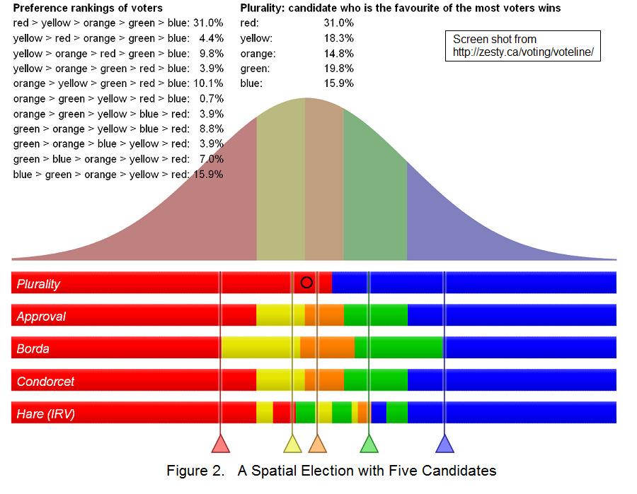
49