Expected Modes of Policy Change in Comparative Institutional Settings * Christopher K. Butler and Thomas H. Hammond

Transcription

1

2 Expected Modes of Policy Change in Comparative Institutional Settings * Christopher K. Butler and Thomas H. Hammond Presented at the Annual Meeting of the American Political Science Association, Washington, D. C., August Department of Political Science Michigan State University * We used Microsoft Excel to set up the simulations and used Decisioneering s Crystal Ball to run the simulations and to generate the forecasts of our analysis variables. The first author acknowledges Karin M. Butler for help in thinking through some of the simulation mechanics.

3 Expected Modes of Policy Change in Comparative Institutional Settings Abstract In the literature of comparative politics is often argued that presidential systems (as in the U.S.) exhibit greater policy stability, ceteris paribus, than parliamentary systems (as in the U.K.). This suggested empirical regularity has been attributed to the multiple veto points of presidential systems that make policy change "difficult" while parliamentary systems have fewer veto points, making policy change "easier." Elsewhere, we have argued (Hammond and Butler 1996) that merely focusing on institutional rules as the multiple-veto-points argument does does not completely specify the underlying situation. In particular, we argue that policy change is produced by an interaction of institutional rules, preference profiles, and the location of the initial status quo. As such, there are conditions under which two institutional systems should be expected to exhibit the same "mode" of policy change, whether it is incremental change, oscillating change, random change, or policy stability. While these conditions do explain why presidential systems sometimes undergo great policy changes and why parliamentary systems sometimes exhibit great policy stability, they do not explain the empirical regularity advanced in the literature. The purpose of this paper is to investigate the extent to which we should expect to see greater long-run stability in presidential systems than in parliamentary systems. We assume a basic unidimensional spatial model of legislative voting under several different institutional rules. Rather than focusing solely on the number of veto points, we also concern ourselves with preference profiles and the location of the initial status quo. Holding preference profiles constant across institutions, we can determine whether the institutions will produce similar or dissimilar policies. In our previous paper (Hammond and Butler 1996), we made one-period static comparisons and two-period dynamic comparisons. Our examination demonstrated that different systems can produce similar policies and exhibit similar modes of policy change. In this paper, we make multi-period dynamic comparisons among institutional systems. By constructing a common history of preference-profile changes and using these profiles in computer simulations, we approximate the frequency of each mode of policy change for each institutional system examined. While these simulation results demonstrate greater stability for presidential systems than for parliamentary systems in the long-run, they also show that different institutional systems not infrequently exhibit the same mode of policy change. This paper emphasizes the shortcomings of purely institutional-rule arguments while proposing an alternative argument that explains both the long-run empirical regularity of differences in policy stability as well as the occasional short-term similarities. Thus, our argument represents an advance over the existing argument since it explains everything that the existing argument explains but also explains things that the existing argument cannot.

4 Introduction Since the status quo is greatly advantaged in all decisions [in the United States], stability is commonly observed; but, again, it is a random stability based on the pre-existing status quo and the particular set of representatives inherited from the last election. There will be many cycles of opinion in society and many, but fewer, cycles of opinion in the legislature. But there will also be equilibrium imposed simply by the fact that it is difficult to get an extraordinary majority together. In that sense, institutions and the dead hand of the past along with, occasionally, the values of people in society influence outcomes. And any particular outcome is some unpredictable combination of influence from the values of the past and values of the present. (Riker 1986, 147). The advanced industrial democracies appear to show some degree of variation in the public policies they have adopted. Parliamentary systems, for example, generally have somewhat more expansive social welfare programs than does a separation-of-powers system like the United States. The advanced industrial democracies also appear to show some degree of variation in the patterns of change in these public policies. Policy changes in the Westminster democracies sometimes appear to show a substantial degree of back-and-forth oscillation as control of the government shifts back-and-forth between labor governments and conservative governments, while the separation-of-powers democracies are more likely to exhibit long periods of policy stability, marked by occasional bursts of large-scale policy change. A wide variety of factors have been advanced as accounting for these differences in the policy choices and in the patterns of policy change of the advanced industrial democracies. One broad set of factors, of enduring interest to students of comparative politics, though perhaps of greater interest in the 1950's and 1960's than more recently, involves differences in political culture and public opinion (Almond and Verba 1963; Abramson and Inglehart 1995) among these countries. While the notion that citizens in any one industrial democracy all share pretty much the same political culture has come under attack, there is continued interest in the extent to which public opinion is homogeneous or heterogeneous, and in the extent to which voters are divided into cohesive blocs based on religion, race, class, or ethnicity (see, e.g., Lijphart 1977). 1

5 A second set of factors, also of enduring interest to students of comparative politics, involves the countries' electoral laws and the party systems that result. Different electoral laws e.g., single-member majority-winner districts versus proportional representation are thought to produce different numbers of parties (Rae 1967, Lijphart 1990), and the number of parties in turn likely affects whether national policies are adopted by just the members of some majority party, or whether policies must be negotiated among a number of parties (Grofman and Lijphart 1986). A third set of factors, much in vogue in recent years, involves differences in the political institutions comprising these countries. Many institutional differences may be important, involving such matters federalism versus unitary government, the extent of independence of the court system, and the number of independent centers of authority in the legislative process (Lijphart 1984, Shugart and Carey 1992, Weaver and Rockman 1993). This last factor has probably attracted the most attention, and recent studies (see especially Tsebelis 1995) have advanced the argument that the number of separate institutions with authority to veto policy changes has a fundamental impact on the nature of policy change, or lack thereof, in the advanced industrial democracies. A fourth set of factors, which have received considerably less attention than the others, involves the argument that the policies adopted by a country are not "path independent" but instead are "path dependent". That is, "history matters": the policies which a country adopts are affected by the policies which the country previously adopted (Lindblom 1965, North 1990, ch.11). It is difficult to maintain and argument that any one of these four sets of factors is unimportant. Yet there have been few efforts to assess the relative importance of these various kinds of factors. Of course, any such assessment raises difficult conceptual and methodological issues. Among them is the likelihood that these various factors do not affect policy independently of the others; that is, their impacts are probably not additive but instead are 2

6 interactive in some complex fashion. Yet having said this, the precise nature of these interactions must be specified before any kind of empirical test is possible. Informal reasoning is unlikely to clarify the precise nature of these interactions; this difficult task is one for which formal theory is likely to be needed, and in a prior paper see Hammond and Butler (1996) we developed a series of formal models of different kinds of democratic political systems. We then used these formal models to make some systematic comparisons of the policy choices which were feasible in the systems, as well as some systematic comparisons of the patterns of policy stability and policy change expected from the various systems. However, some kinds of comparisons across systems were not easily amenable to formal analysis. In particular, we were sometimes able to tell via formal analysis whether a pair of systems could, in principle, produce similar or dissimilar results, but we could not easily determine the extent of similarity or dissimilarity in results which should be expected on average. For this reason we have resorted to computer simulation. We constructed computer models representative of the range of democratic political systems characterized in Hammond and Butler (1996). We then systematically manipulated each variable, while holding constant the other variables, so as to determine the extent of impact on policy choice and policy change. The results from this kind of sensitivity analysis provide a foundation on which more refined judgments can be made about the relative importance of the various sets of factors which affect policy choice and policy change, and may also contribute to the specification of more refined empirical tests. Simulation Setup Before conducting our analysis, several procedural considerations need to be settled. As our major goal is to produce comparability among systems, let us focus the reader s attention here. Our argument is that institutional rules alone do not produce similarities (or differences) in modes of policy change. Instead, policy change stems from a complex combination of preferences, changes in preferences, the location of the initial status quo, and institutional rules. 3

7 The problem with comparative analysis addressing the issue of stability is that no one of these aspects is necessarily comparable across systems in the real world. For instance, presidential systems are argued to be more stable than parliamentary ones ceteris paribus, but this is only a partial analysis. If preferences remain constant over time in a parliamentary system, stability will be the result. But the same could be true in a presidential system, as well, without using multiple veto points in the explanation. Within a simulated environment, we can control two of our three vital components: individual preferences and the location of the initial status quo. This allows us to examine the independent effects of institutional rules; that is, we can truly hold all else equal. We accomplish this task along a unidimensional issue space, which we bound between 0 and 100. Hence, the initial status quo, SQ 0, is merely a number in that range. The same SQ 0 is used for each of the systems analyzed. Preferences in unidimensional space are also represented by a single number for a single person at a moment in time. The notion of a preference profile (Arrow 1951) in this space is merely a vector of individual preferences at a moment in time. We will distinguish between two concepts that naturally follow from this. The first is a preference history. This is a vector through time of preferences associated with a particular legislative seat or presidential office. The second concept is that of a profile history. Abusing language, this is a vector of preference profiles through time. This amounts to a matrix in which each row is a preference profile and each column is a preference history. It is the profile history that is our main vehicle of compatibility among systems since we can generate one profile history and use it in the analysis of each system. In the pages that follow, we list the legislative systems to be analyzed. We then discuss our independent variables in greater detail. After that we discuss our dependent variables. Most of these follow from the nature of spatial modeling. We do, however, construct several new 4

8 measures of policy change and stability. We then review how each system is modeled in the simulation and, more importantly, how specific policies are chosen in each period. SYSTEMS TO BE ANALYZED. We analyze the modes of policy change in each of the legislative systems discussed in Hammond and Butler (1996) plus one new system. These systems are (1) a unicameral two-party system, (2) a unicameral coalition-party system with three parties, (3 & 4) a bicameral system with and without parties, and (5 & 6) a tricameral system i.e., a bicameral system with a president with and without parties. These simplified systems represent the essential qualities of many real-world legislative systems. We do not formally analyze the unicameral party-free system, but we do use the underlying median voter as a benchmark in some of our analyses. 1 BASIC INDEPENDENT VARIABLES. As mentioned above, our main concern is that comparative analysis of institutional rules makes sense in a quasi-experimental setting. This requires that preferences and the initial status quo, SQ 0, be the same across every system. To accomplish this, we randomly generate a profile history containing thirteen preference histories under three different assumptions. The first assumption is that preferences are drawn from a uniform distribution having its mean at 50 and endpoints at 0 and 100. The second assumption is that preferences are drawn from a normal distribution also having its mean at 50 but having a standard deviation of 16. This gives an empirical range close but somewhat larger range than that of the uniform distribution; however, this larger range does not present a problem since so few preferences are drawn from the extremes of that range. The third assumption is that assumptions are drawn from a bimodally normal distribution also having its mean at 50. The two modes are centered on 25 and 75 and have standard deviations of 8 from these points. This distribution also has a range close but somewhat larger than that of the uniform distribution but smaller that that of the normal distribution. Again, fewer preferences are drawn from the extremes of this 1 The notion of a party-free system could also be construed as a single-party system. 5

9 distribution than in the uniform case. The assumptions regarding the distribution of preferences is the closest approximation we have for political culture. The uniform distribution represents a rather diffuse population of political opinion while the normal distribution represents a significant degree of agreement on political issues. The bimodal distribution represents a factionalization of political opinion but general agreement within the factions. The choice of thirteen preference histories is based on the systems under study. For our tricameral system with two parties, we wanted there to be enough possible divisions of party within each chamber to create a variety of circumstances. With thirteen preference histories, we can have a house with seven members and a senate with five members plus the president. This also produces a single median in each chamber of the tricameral system, reducing computations. In dividing a unicameral legislature among three parties we desired sufficient variation of possible coalitions. With thirteen preference histories, the most equally divided system can have a split and numerous other combinations of two and three parties. In our selection of a common SQ 0, we wanted to test another conjecture: that the SQ 0 can affect the history of policy change in a system. To this end we ran five separate simulations on each system using five different but common SQ 0 s. Recall that our unidimensional system is bounded between 0 and 100. Our five common SQ 0 s are 0, 25, 50, 75, and 100. Since we had identical profile histories, we expect policies to converge to some identical sequence of policy changes over time. However, we also expected that the rate of convergence would depend on the institutional rules in question. For instance, convergence is immediate in the basic unicameral party-free system. We will discuss this aspect of the analysis in greater depth later in the paper. Selection of the common SQ 0 provides two useful things. The first already mentioned is testing how much the initial status quo matters within different systems. The second is a check on the simulation results. Specifically, we expected a given system to exhibit 6

10 the same modes of policy change despite having different SQ 0 s. This is especially important during the period of convergence. If modes of policy change are significantly different during this period, then the simulation results are suspect. Hence, we operationalize diagnostics to check for this. DEPENDENT VARIABLES. Our principal endogenous variable is the policy along the issue space that results from the interaction of initial status quo, the preference profile, and the institutional rule. This variable the resultant policy at time t is designated as SQ t. Although the very first initial status quo has been experimentally selected, the initial status quo of each subsequent period is determined by the previous resultant policy. Thus, SQ t 1 is the initial status quo for time t. Within the simulations, we have two vectors representing policy choices SQ t 1 and SQ t representing the initial and resultant status quo points respectively. The first element of SQ t 1 is the independent variable SQ 0. How SQ t is determined in each system is discussed in detail in a subsequent section. Merely comparing resultant policies between systems does not capture the essence of modes of policy change. Hence, we do not use SQ t by itself in comparative analysis. 2 Instead, we make use of two different variables and time-series techniques. The first variable is the magnitude and direction of per period policy change namely SQ SQ t SQ t 1. This variable captures some features of stability and is comparable between systems. The other variable marks the magnitude and direction of resultant policies from the system median ( ~ x t ) namely ~ x SQ ~ x. This represents the effect of institutional rules on policy using the overall median as the baseline. t 2 We do, however, use SQ t to analyze convergence within systems. 7

11 While SQ captures both magnitude and direction of policy change, it does not get at the frequency of policy change. We examine three frequency variables. The first starts as a simple dichotomous variable of per-period stability, v t, that is 1 if SQ t 0 and is 0 otherwise. T vt t The average per period frequency (i.e., V 1 ) provides an estimate that is comparable across T systems and that is intuitively grasped as the expected probability of policy stability in any given period. The above measure, albeit intuitive, is quite sensitive. Any policy change no matter how small decreases the average frequency of stability. Although this is fine in theory, in practice small changes in policy are almost imperceptible. To filter out these small changes, we have constructed two epsilon measures. The first is an extension of the measure above. In it, v t 1 if SQ t vt t and is zero otherwise. The frequency measure is then V 1. When T T 0, this measure is the same as above. We also examine V at = 1, 5, and one standard deviation of SQ t. This provides us with three absolute measures of comparison when using = 0, 1, and 5 as well as one relative measure when using a system s own standard deviation of policy change. This relative measure may be likened to someone measuring perceptible changes given the context of a particular institutional setting. The second epsilon measure, W, examines the duration of stability by asking how many consecutive periods has policy been within of the current policy. Thus, for = 0, w t is the number of periods leading to period t for which there has been no policy change. W 0 w t 1 is the expected duration of any specific policy. For 0, w t is the number of T t T 8

12 periods leading to period t for which policy was within the zone SQ t. We calculate W for the same values of as we did for V : 0, 1, 5, and the standard deviation of policy change. As we are interested in modes of policy change rather than merely degrees of stability, we have developed a categorical per period variable that examines local trends in policy change. Recall that we have distinguished three different modes of policy change namely incremental change, oscillating change, and periods of stability. When considering what these modes of policy change might look like, one realizes that there are also many sequences of change that are not easily categorized. The problem is identifying systematic change (or stability) from noise. The variable we have created is based on the direction of change (but not the magnitude of change) for the previous five periods. Analyzing with respect to time t, we examine the sequence sign SQ t 4, sign SQ t 3, sign SQ t 2, sign SQ t 1, sign SQ t. This sequence contains the elements {-1, 0, 1}. Since the sequence has four components, there are 81 possible sequences that represent local trends in policy change. We have categorized these sequences in the following way. Stability is represented by any sequence with three or more zero elements. There are nine such sequences. Incremental change is represented by (1) three -1 elements and a zero in any order, (2) three 1 elements and a zero in any order, (3) four -1 elements, or (4) four 1 elements. There are ten such sequences. Oscillating change is represented by (1) the elements -1, 1, -1 in order with a zero interspersed at any point, (2) the elements 1, -1, 1 in order with a zero interspersed at any point, (3) the sequence -1, 1, -1, 1, or (4) the sequence 1, -1, 1, -1. There are ten such sequences. The remaining 52 sequences are labeled as noise. The above measure provides a systematic yet convenient method of comparing the results of different systems. By producing three relevant frequencies (as percentages) for each system, this measure greatly simplifies comparison and allows us to get to the root of our inquiry. It gives a simple but direct answer to the question, What is the expected mode of policy change in a 9

13 system? At the same time, however, it addresses the likelihood of each model of policy change. Although nearly 65% of the possible sequences have been categorized as noise, the usefulness of the measure is based on two key points. First, the same measure is being applied to each system, and each system has the same profile history. Thus, in the absence of (complex) institutional rules, the measure would give the same result time and again. This provides an underlying uniformity not known in most empirical investigations. Second, we have identified selected sequences because they clearly belong to a particular category. If we had categorized each sequence as incremental, oscillating, or stable without a noise category, we would have do so under ad hoc assumptions. Instead, we opted to create systematic categorizations grounded strictly on an interocular basis i.e., if a sequence doesn t hit you between the eyes as belonging to a certain category, don t put it there. SYSTEM SPECIFIC VARIABLES. Having described the variables common to each system, it is now appropriate to describe variables specific to different systems. These variables involve the actual modeling of each system. In addition, the system specific variables are important determinants of the resultant policy for each preference profile. The exact method of determining the resultant policies in each system is discussed in the next section. The importance of system specific variables cannot be understated. Given the most basic system a unicameral party-free legislature one only needs to know the current preference profile and then apply the median voter theorem (Black 1958). The systems we model, however, require greater deliberation. The existing status quo becomes important whenever the core is larger than one point. The core is the set of policy points that cannot be upset under the institutional rules (c.f., Hammond and Miller 1987 and also Debreu and Sharf 1963; Gillies 1953, 1959; Shapley and Shubik 1971; Shubik 1959). 3 If the existing status quo is outside a new core, several factors affect where in the core the resultant policy would end up. For the systems 3 Perhaps the best intuitive definition is found in Shapley and Shubik (1971, 2) where the core is defined as the set of outcomes that no coalition can improve upon. 10

14 analyzed here, the two factors we model are chamber and party membership. Chamber membership is a consideration in four of our systems. Since each of our thirteen preference histories are randomly generated independently of each other and, especially, of its relative location in the preference profile, it is sufficient to specify that a particular preference history represents a seat in one of the two (or three) chambers. For all analyses of bicameral legislatures, we let the first six preference histories comprise one chamber while the remaining seven preference histories comprise the other chamber. Similarly, for all analyses of tricameral legislatures, we let the first preference history represent the office of the president, the next five preference histories comprise the first chamber, and the remaining seven preference histories comprise the second chamber. The other factor that affects the resultant policy is party membership (in combination with assumptions about party discipline, discussed later). Two methods are used to determine party membership. The first method presumes contiguity of membership. Under this method, we merely generate a random integer L from 0 to 13 for each preference profile that represents the number of members in the left-most party. If there is a middle party, we generate another random integer G from 0 to 13 L. That represents the number of members of the middle i.e., Green party. The number of right-most party members R is the remainder 13 L from the left. G. Party membership is then assigned along the underlying dimension by counting The other method of deciding party membership employs a completely random assignment of each preference. Thus, this method minimizes the possibility of contiguity. By employing such an extreme mechanism, we can separate the effects of party discipline alone from party discipline with underlying contiguity. Since neither method relies on chamber membership, they can be computed once per method for each of the two-party systems. This allows us another element of ceteris paribus. 11

15 Specifically, party membership will matter, but the division of party membership will be the same in each two-party system. If the division of party membership were different between systems, differences in the modes of policy change could be attributed to this aspect rather than more appropriately attributed to institutional rules. Our conception of party discipline revolves around agenda control. Parties have some degree of consensus regarding what policy to implement. This consensus may be divided due to chamber membership but even then party caucuses develop chamber agendas. In either case, a party platform is determined by the median position of relevant members. When there is an even number of party members, we allow for a range of policies that make up the core of the party caucus. The preceding discussion outlined the basic variables necessary in the computation to resultant policies. Several intermediate variables beyond the above are also necessary. Most of these are mentioned in the next section. SYSTEM SPECIFIC PROCEDURES. In this section we lay out the specifics of determining resultant policies in each of the analyzed systems. There is, however, a general outline employed in each case. First, we determine the core in each period. If the existing status quo is contained in this core, then the resultant policy is the same as the existing status quo. If not, then the resultant policy is contained within the intersection of the core and the win set off the status quo of the legislator 4 closest to the status quo and whose ideal point is still contained in the core. win set SQ t-1 core SQ t in here Consider the above diagram. In this diagram the existing status quo, SQ t 1, is located to 12

16 the left of a line core represented by the gray box. There is at least one legislator at the leftmost boundary of the core. The boundary of the win set off the status quo of this legislator is graphed above the issue dimension. The core covers part of this win set. The region of intersection represented by the line segment below the issue dimension will contain the resultant policy, SQ t. Note that this region may be the entire core if SQ t 1 is far enough away from the boundary legislator. Once the potential region of the resultant policy is found, the requirements of the simulation demand that a particular point within this bounded region be selected as SQ t. Hence, the following subsections are devoted to answering two questions. First, how is the core defined in each system? Second, if the resultant policy needs to be selected from a range of policies, what is the exact procedure for this? To facilitate this procedural discussion, it is helpful to introduce some notation. First, recall that SQ t 1 is the existing status quo and that we are trying to pinpoint SQ t, the resultant policy. Each of these is a singe point in unidimensional space between 0 and 100. Denote core as the set of stable policy positions belonging to the core. Note that core will always contain at least one point in unidimensional space. Two factors are important when considering an individual legislator s position party and chamber. Denote a particular legislator by x n ij where i L, G, C, j H S P,,, and n is a numeric index of legislators having i and j in common, party is represented by i (Liberal, Green, and Conservative) and chamber is represented by j (House, Senate, and President). In this way, x ij represents the set of legislators having characteristics i and j in common. Extending this notation, let a ij represent the agenda of x ij. This is synonymous with the median of the 4 Although we use legislator throughout when discussing members of the system, we include the president (in the tricameral systems) as a legislator. 13

17 unicameral party-free core of x ij. Once we have found the core, we will often need to know the *, 1 be legislator nearest SQ t 1 but still in the core. Denote this legislator as x * and let Wx SQ t x * s preferred-to set off SQ t 1. Finally, let Ix *, SQ t 1 be Wx SQ t *, 1 core. Unicameral two-party system. In this system we only have x L and x C. One of these two parties will have a majority in the chamber. The core of this system is the same as the agenda of the majority party. When SQ t 1 is outside the core of this system, SQ t is selected to be the midpoint of the line segment Ix *, SQ t 1 where x * will be a member of the majority party. Unicameral three-party system. In this system we have x L, x G, and x C and must consider two possible cabinet types. On the one hand, one of the three parties may have a majority. In this case, the identification of SQ t is the same as in the unicameral two-party system. On the other hand, no single party may enjoy majority status. In this event, we require that the coalition be a minimum winning connected coalition following Axelrod (1970, ; see also Riker 1962). Since we only have three parties, this assumption implies that the Green party is part of any coalition when a coalition government is necessary (see Axelrod 1970, p. 170ff). We examine the size of the two possible coalitions namely x LG xl xg and x x x GC G C. Since the governing coalition must have a majority of the chamber, we check for this property first. If only one coalition represents a majority, then that coalition is the governing coalition. If both x LG and x GC represent majorities of the system, then we select the smaller to be the governing coalition. In the rare event that both x LG and x GC represent majorities of the system and are of the same size, the governing coalition is selected at random. After determining the governing coalition, we must consider the separate agendas of the two member parties. Rather than assuming that the coalition members create a coalition agenda e.g., the median of the coalition we assume that any change in policy must be 14

18 agreeable to both parties. This has the effect of making the coalition members function as a bicameral subsystem. As such, the core of the system is the entire range of policies between and including the agenda of both parties in the coalition. Once the coalition core is found, SQ t if outside this core is the midpoint of the line segment Ix *, SQ t 1. Bicameral party-free system. In this system we have x H and x S, representing House and Senate members. Each chamber, like our parties, has its own agenda a H and a S represented by the median member of the House (having seven members) and the unicameral core of the Senate (having six members). The system core is the unbroken line segment that covers both agendas. If SQ t 1 is outside this core, then we take SQ t as the midpoint of the line segment Ix *, SQ t 1. Bicameral two-party system. For this system we must deal with four groups of legislators: x LH, x CH, x LS, and x CS. Recall that x H has seven members while x S has six members. This ensures that the House will have a party with a clear majority. Identify this party as x mh. If one party has a clear majority in the Senate, identify this party as x ms. In the event that there is an even split in the Senate, we take the Senate agenda as the unicameral party-free core of the senate. The main difference between this system and its party-free counterpart is the selection of agendas in the chambers. The agenda of a chamber, a, is the unicameral party-free core of x m. Since party membership fluctuates, a need not be a point in either chamber. The core of this system is again the unbroken line segment that covers both agendas i.e., a H and a S. Once the core is found, selection of SQ t is the same as in the bicameral party-free system. Tricameral party-free system. In this system we have x H with seven members, x S with five members, and x P being an individual. Each chamber has an agenda represented by the median member. The core of this system is the line segment that connects the outermost agendas. 15

19 If SQ t 1 is outside the core, we again take SQ t as the midpoint of Ix *, SQ t 1. 5 Tricameral two-party system. Like the bicameral two-party system, the chamber agendas are functions of the majority parties. Since the House has seven members and the Senate has five members in the tricameral system, each will have a clear majority party x mh and x ms. The agenda of each chamber is the unicameral party-free core of its majority party. The system core is then the unbroken line segment that covers a H, a S, and x P. Selection of SQ t is then conducted under the same method as in the tricameral party-free system. Results and Findings To examine policy changes in the above systems we created a spreadsheet representing a history of one hundred electoral cycles and calculated our various dependent variables for each system. The data reported here are averages over one hundred trials, each representing a history of one hundred electoral cycles. As such, we are able to report point estimates and standard deviations of these point estimates. With only one hundred trials, however, we consider our results tentative with respect to significant differences between point estimates. The results are reported in the following manner. First, we examine differences within systems with respect to the initial status quo and the underlying preference distribution. This examination is noteworthy for its general lack of differences, but some surprises emerge. Second, we examine differences between systems while holding the initial status quo and the underlying preference distribution constant. This analysis is mostly confirmatory but is remarkable in how stark some of the differences are. Finally, we analyze policy convergence for six of our systems. Again, what we find is mostly confirmatory but we do witness some variation caused by the underlying preference distribution and party discipline. This analysis is augmented by 5 We realize, of course, that this assumption is likely to be the most sensitive in the tricameral system for the selection of SQ t. It would be interesting to examine the impact of varying agenda setters in this institution. 16

20 descriptive statistics regarding the sizes of cores and the frequency of having point cores in the different institutional systems. Given the wealth of data, we will refer to variable specific tables for the first two sections of analysis. Table 1 summarizes our modes-of-policy-change variables of incremental and oscillating change as well as stability. Since these variables depend on the previous four periods to make per-period observations, each trial mean is calculated over 96 electoral cycles. Table 2 summarizes the frequency of stability. This represents our V measures. Tables 3 and 4 summarizes our W measures for the duration of stability. Table 3 reflects mean durations while table 4 captures the longest sequence of stability over one hundred electoral cycles. Table 5 summarizes various deviations in policy change. The three variables on this table are the mean (absolute) deviation from the underlying system median, the mean (absolute) size of per-period policy change, and the standard deviation of policy change. This last variable reflects the average of the standard deviations used in V sd and W sd. DIFFERENCES WITHIN SYSTEMS. Although we have been gearing up to examine policy change between systems, our argument throughout is that the type and frequency of policy change results from a confluence of institutional rules, preferences, and the location of the initial status quo. Given the quasi-experimental control of our simulation, we can analyze the independent effects of each of the elements above. Thus, before we examine the effects of institutional rules we will discuss the effects of the other elements within particular institutional arrangements. This is similar to the comparativist endeavor of analyzing individual countries with respect to political culture represented in part by our preference distributions and history reflected by the location of the initial status quo. Rather than going system by system, however, we are looking for regular results occurring in variables. We first examine the effects of the initial status quo. Overall, the location of the first status quo has only minimal impact on our dependent variables. In fact, only two variables 17

21 register any statistical effects 6 and only in combination with normally distributed preferences. These are the frequency of stability with the lowest sensitivity (V sd ) and the standard deviation of policy change. Since the standard deviation of policy change affects V sd, let us examine that variable first. When preferences are normally distributed, the location of the initial status quo has a fairly consistent effect on the standard deviation of policy change (see table 5). Specifically, the simulations using 50 as the first status quo tend to have a lower standard deviations of policy change than simulations using 0 or 100 as the initial status quo. This seems to suggest that systems with moderate beginnings and homogeneous culture are likely to experience smaller changes in policy than a homogeneous culture with extreme beginnings. The above result has a secondary effect on the frequency of stability when using the standard deviation of policy change as a gauge to stability. Since the simulations using an initial status quo of 50 have smaller standard deviations of policy change than the other two simulations, the V sd measure is more sensitive to policy change in these simulations. The fact that this difference only shows up for normally distributed preferences is likely to be related to the normal distribution having a greater central tendency than the other two distributions. Hence, starting in the middle of the spectrum, a system with an initial status quo of 50 is likely to experience greater stability prior to convergence i.e., the time at which different histories produce the same policies. The fact that the differences are greatest with the tricameral systems lends some support to this possibility since the tricameral systems take longer to converge, giving time for differences in stability to make their mark on the final summary statistic. V sd (see table 2) approaches significance (i.e., 0.05 < p < 0.10) for three systems: unicameral two-party with random party membership, bicameral party free, and tricameral party free. In each of these systems, the simulation using an initial status quo of 50 yielded smaller 6 All statistical analysis involves difference of mean estimates using the Student s t-distribution (twotailed) with 99 degrees of freedom. 18

22 frequencies of stability than either of the other two simulations (starting with initial status quo points of 0 and 100). This is due more to the differences in standard deviations of policy change noted above and is not necessarily an independent result since the V sd measure is more sensitive to change for moderate histories. The underlying distribution of preferences has a greater effect on policy change. For policy changes larger than five units (i.e., looking at V 5 on table 2), normally distributed preferences have greater frequencies of stability than either bimodal or uniform preferences within unicameral and party-free systems. When allowing for a greater window of policy change (i.e., looking at V sd ), bimodal preferences have a lower frequency of stability than either normal or uniform preferences within unicameral systems. This suggests that more homogeneous political cultures produce more policy changes that are moderately imperceptible than those produced by heterogeneous political cultures. No distributional effects are present on V 0 or V 1. Thus, all cultures make some kind of policy change with equal likelihood. A similar result appears when we examine the mean duration of stability (see table 3). For W 5, normal preferences have a consistently longer duration of stability than uniform preferences in unicameral systems. In the unicameral two-party system with random party membership, we see that normal preferences also have a longer duration of stability than bimodal preferences. This is hardly surprising since it is the same as saying that highly homogeneous political cultures have longer periods of stable policies than more disperse cultures. However, this is only true in unicameral systems. The underlying distribution of preferences does not affect the maximum duration of stability in any system or the duration of stability in multiple veto-point systems. This implies rather strongly that political culture plays no meaningful role in determining when policies are likely to change in bicameral and tricameral systems. Bimodal preferences yield consistently larger per-period deviations in policy (see table 5) than do normally distributed preferences. The same is true for uniform preferences. This says 19

23 that more heterogeneous cultures have larger changes in policy on average than more homogeneous ones. Bimodal and uniform preferences generally follow similar patterns except in deviations from the underlying median. For the unicameral three-party (random) system, all bicameral systems, and the tricameral party-free system, bimodally distributed preferences deviate more from the underlying median than do uniform preferences. The most remarkable result when looking for within-system differences is that our modes-of-policy-change measures are in no way affected by preference distributions or the initial status quo (see table 1). This emerges despite the differences already noted in the other variables. In fact, the smallest p-value in the analysis of within-system differences for stability and incremental and oscillating change is This clearly suggests that the underlying preference distribution and the initial status quo does not have long-standing effects on modes of policy change. Although political culture and history have some effects on the frequency and size of policy change, they have no impact on the type of policy change in a given system. SYSTEM DIFFERENCES. Now that we have examined the effects of preferences and the initial status quo, we can explore the independent effects of institutional rules with greater confidence. Recall that our modeling of institutional arrangements consists of two components. The most prominent component, the number of veto points, has predictable and pronounced effects on all aspects of policy change. The other component, party discipline, also affects policy change but does so in more subtle ways. When looking at differences between systems, we see many confirmatory results. In general, bicameral systems are more stable than unicameral systems, and tricameral systems are more stable than bicameral systems. This shows up on our stability measure (table 1), the frequency of per-period stability (table 2), and the duration of stability (tables 3 and 4). [Figure 1 about here] In figure 1 we have plotted our modes-of-policy-change measures as averages over 20

24 preference distribution and initial status quo. The x-axis in this figure (and all others) represents the ten different systems under consideration. As such, the axis is categorical but is arranged with unicameral systems to the left, bicameral systems in the middle, and tricameral systems to the right. For our stability measure (indicated by the triangles) it is quite easy to see major jumps between unicameral, bicameral, and tricameral systems. There are also consistent and corresponding drops in oscillating change when moving from unicameral, bicameral, and tricameral systems. Although the drop in oscillation from the bicameral to the tricameral systems is small, when comparing like systems we see that the drop from bicameral party-free to tricameral party-free is not significant, but the drops from bicameral to tricameral contiguous and from bicameral to tricameral random are significant. Incremental change registered no meaningful patterns across systems. Although the frequency of incremental change decreased from uniform to bicameral to tricameral systems, these drops in value were not consistently significant. Recall, however, that there is no underlying trend in the preferences being drawn. Hence, we did not expect to see much in the way of incremental change. In future analysis we will incorporate a trend in preferences to examine whether this inverse relationship between oscillating change and veto points continues to hold. One feature that stands out on figure 1 is that the unicameral three-party (random) system is significantly different from the other unicameral systems on both the stability measure and the oscillating-change measure. Upon reflection, we believe that what is actually going on is that both unicameral three-party systems should have greater stability and less oscillation than their two-party counterparts following from Tsebelis s argument that multiple parties in a unicameral system act as multiple veto points (1995). The lower stability and greater oscillation of the unicameral three-party system with contiguous party membership may be an artifact of our party selection mechanism. Recall that contiguous party membership is determined by generating a 21

25 random integer between 0 and 13 for the number of Liberal members. This means that roughly one fourteenth of the time the Liberal party will control all of the legislative seats. For random party membership this figure occurs only once in over 1.23 million electoral cycles. Our average estimated probability of having a point core in the three-party system with contiguous party membership is while the same average for the random-assignment counterpart is only Furthermore, real-world observations of single-party domination of multiparty systems are quite rare. This suggests that our random party membership systems may be a more accurate reflection of reality with respect to observed policy changes. This same jump in stability between the three-party systems is present when measuring the frequency of stability (figure 2) and the duration of stability (see figure 3 below). [Figure 2 about here] In figure 2 we have plotted the average frequency of stability across systems for our four frequency measures. Again, we see the general increasing trend from unicameral to bicameral to tricameral systems. The interesting feature of this figure is that the V sd measure does not have the pronounced jumps of the other three measures. Nevertheless, the significance patterns in pairwise comparisons are the same for all four variables. In figure 3 (below), we see that the positive relationship between duration of stability and number of veto points is again confirmed. [Figure 3 about here] Figure 4 (below) shows the average deviations in policy change across systems. Not surprisingly, we see that the average policy change (and its standard deviation) is inversely related to the number of veto points. Although small, the difference between bicameral and tricameral systems is small but significant when comparing the two-party systems. The party-free systems, however, do not register significant differences. Once again, the two three-party systems deviate significantly from one another on these two measures. [Figure 4 about here] 22

26 Deviations from the underlying median are more difficult to interpret. It is clear that the existence of disciplined parties has an impact on policy. This observation is borne out in large differences from zero for the unicameral systems as well as significant jumps from party-free to two-party systems in both the bicameral and tricameral cases. In fact, the most striking movement on the graph is the jump from tricameral party-free to tricameral two-party. It is not necessarily clear whether more veto points leads to greater deviations from the underlying median. POLICY HISTORY AND CONVERGENCE. While we agree that history matters on the development of specific policies, we wonder how much history matters. Specifically, we examined how quickly policy series converged given different initial status quo points. The rate of convergence within a system is an inverse measure of how long a history of policy changes can remain independent from some other history of policy changes. Convergence of this type requires that the underlying preferences be identical for policy histories with different starting points. Identical preferences make convergence possible and, once convergence is attained, the policy histories will have identical policy movements. This analysis only examines the partyfree and contiguous-party-membership systems. For each preference distribution and legislative system combination we used initial status quo points of 0, 25, 50, 75, and 100. This gave us ten pairwise comparisons to consider. After calculating series convergence for each pairing, we calculated three main summary measures. The first of these is partial convergence. This is the minimum of the pairwise calculations and represents the first point at which any two series converged. The next measure is total convergence. This is the maximum of the pairwise calculations and represents the point at which all five series converged. Finally, we also calculated the difference between total and partial convergence. This provides a rough estimate of how long it takes for total convergence after two series converge. Table 6 summarizes all of this information. 23

27 [Table 6 about here] The interesting feature of convergence within all of the systems but more pronounced in the multiple-veto-point systems is that series starting with extreme points (e.g., the 0/100 series) converge faster than series with more moderate beginnings. This result is generated by two things. Series with extreme initial status quo points are more likely (1) to be outside the core and (2) to have identical bargaining sets specifically the core itself (i.e., their respective winsets are likely to contain the entire core). Having identical bargaining sets, the resultant policy is generated identically according to our simulation procedures. Hence, this may be an artifact of our selection mechanism. However, we believe that any consistent selection mechanism would produce similar results. System by system we find that unicameral systems converge faster than bicameral and tricameral ones and that bicameral systems converge faster than tricameral ones. This is directly related to the average size of cores within these systems (see table 7 below 7 ). Since bicameral and tricameral systems are likely to have larger cores than unicameral systems, bargaining sets with respect to different status quo points are likely to be incongruous. This leads to longer periods of policies being divergent. [Table 7 about here] The likelihood of having a point core also affects time to convergence. Once a system experiences a point core, all series necessarily converge to that point. Unicameral two-party systems have point cores about 60% of the time, bicameral two-party systems have point cores about 2% of the time, and tricameral two-party systems have point cores less than 0.1% of the time. This leads to much greater latitude for policy divergence in bicameral and tricameral systems. The underlying preference distribution also has some effect on convergence. For the 24

28 bicameral and tricameral systems, normally distributed preferences achieve partial convergence before uniformly distributed preferences while bimodally distributed preferences achieve total convergence faster (though not statistically speaking in either case) than either normally or uniformly distributed preferences. The first result is due to normal preferences generating a smaller core on average than uniform preferences. The second result is more challenging to explain. Although bimodal preferences generate larger cores than normal preferences, they are about as large (on average) as those generated by uniform preferences. Hence, the size of the core probably does not produce this result. It is possible that the large policy changes occasioned by bimodal preferences cause extremist policies. We have already seen how series that start with extreme status quo points tend to converge faster. Thus, while normal preferences are producing partial convergence, bimodal preferences are pushing centrally located policies to the extremes of the spectrum. Once policies are at extremes, total convergence occurs faster than with normal preferences. Conclusion We have argued that variations in policy change are produced by an interaction among institutional rules, legislators' policy preferences, and the initial location of the status quo. The literature on the comparative politics of advanced industrial democracies suggested that each of variables should be expected to influence the extent and nature of changes in public policies, and our simulation produced support for each of these variables. POLITICAL CULTURE AND PUBLIC OPINION. We modeled political culture and public opinion as involving the underlying distribution of preferences from which legislators are drawn. Our results in this area indicate a variety of things. First, a homogeneous political culture is likely to produce smaller policy changes than more heterogeneous political cultures. This is 7 The simulations used to produce table 7 measured the size of the core as the range of its endpoints and the frequency of having a point core as the frequency of having a range of 0. Since these measurements are not dependent on history, we merely simulated a single electoral cycle for 10,000 trials. 25

29 especially true when initial policies are in the middle of the spectrum. Second, highly heterogeneous political cultures have less impact on what history of policy changes are observed in that culture. This is evidenced by the faster convergence of bimodal preferences, meaning that initial differences in policy are likely to vanish more quickly in heterogeneous cultures. On the whole, however, moving from one underlying preference distribution to another did not greatly influence patterns of policy change. PARTY SYSTEMS. We had only one pair of models in which we could compare a twoparty system with a three-party system, with everything else held constant: this involved the twoparty unicameral system and the three-party unicameral system. We found some evidence that multiple parties in coalition acted in the same manner as additional veto points. Specifically, coalitions tended to increase policy stability and decrease policy oscillation. We also found that party discipline had some affect on increasing the frequency and duration of stability. Party discipline also drew policy away from the underlying median. These results provide support for the argument by Tsebelis (1995) that partisan veto points can have the same kind of impact as institutional veto points; in either case, an increase in the number of veto points increases policy stability. We have reason to believe that this impact is greatest in unicameral systems, but only future research will speak to this point. THE NUMBER OF VETO POINTS. The impact of the number of veto points was quite pronounced. Rather predictably, the impact of an increase in the number of veto points was to increase the stability of policy: policies simply tended to remain the same for longer periods of time in tricameral systems compared to bicameral systems, and for bicameral compared to unicameral systems. This was clearly due to the fact that as the number of veto points increased, the size of the core generally increased as well. However, the move from a unicameral system to a bicameral system increased policy stability more than the move from a bicameral system to a tricameral one. Hence, the impact of increased veto points may be asymptotic with respect to the 26

30 degree of stability. Another impact of the larger average size of the cores was that multiple vetopoint systems experience less oscillation of policy. In addition, when policies did change, the policy changes in multiple veto-point systems tended to be smaller than the policy changes in unicameral systems. Thus, not only did multicameral systems produce more stable policies, but they also moderated the size of policy changes. Finally, policy choices in the tricameral systems tended to deviate more from populist expectations i.e., the overall median than did the other systems. THE IMPACT OF HISTORY. Our last set of factors involved the impact of "history". In particular, we examined whether the location of the initial status quo affected subsequent patterns of policy change. We found that, given normally-distributed preferences, the initial location of the status quo could affect the frequency and size of policy change at the margins. In particular, an initial status quo in the middle of the spectrum in combination with normal preferences produced smaller and somewhat less frequent policy changes than an initial status quo toward an extreme end of the spectrum. In contrast, when preferences were either uniformly distributed or bimodally distributed, the location of the initial status quo had a negligible little impact on the frequency or size of policy change. OVERALL. It would be desirable to make some assessment of the "relative" impact of the variables whose values we were able to control or manipulate in our simulations. For the particular ranges of variation which we used for our systems from 1 to 3 institutional veto points, from 1 to 3 parties, three different opinion distributions (uniform, normal, bimodal), and five different initial status quo points (0, 25, 50, 75, 100) changes in the number of veto points appeared to have a greater impact than any other single variable. However, there is no obvious way of "calibrating" these variables so that they are on any kind of "common scale", hence this conclusion about the greater impact of the number of veto points must be treated very cautiously. The reason, of course, is that there may well be values for these other variables which we did not 27

31 examine and which could conceivably have had as much impact as the number of institutional veto points. 28

32 WORKS CITED Abramson, Paul R. and Ronald Inglehart Value Change in Global Perspective. Ann Arbor: University of Michigan Press. Almond, Gabriel and Sidney Verba The Civic Culture. Princeton: Princeton University Press. Arrow, Kenneth J Social Choice and Individual Values. New Haven, CT: Yale University Press. Axelrod, Robert Conflict of Interest, A Theory of Divergent Goals with Applications to Politics. Chicago: Markham Publishing Company. Black, Duncan Theory of Committees and Elections. Cambridge: Cambridge University Press. Debreu, Gerard and Herbert Scarf A Limit Theorem on the Core of an Economy. International Economics Review 4: Gillies, Donald B Some Theorems on n-person Games. Princeton: Princeton University, Ph.D. Dissertation. Gillies, Donald B Solutions to General Non-zero-sum Games. In Contributions to the Theory of Games, A. W. Tucker and R. D. Luce, eds. Princeton: Princeton University Press. 40, IV. Grofman, Bernard and Arend Lijphart, eds Electoral Laws and Their Political Consequences. New York: Agathon Press. Hammond, Thomas H. and Christopher K. Butler Some Complex Answers to the Simple Question, Do Institutions Matter? : Aggregation Rules, Preference Profiles, and Policy Equilibria in Presidential and Parliamentary Systems. Midwest Political Science Association, Chicago, IL. Hammond, Thomas H. and Gary J. Miller The Core of the Constitution. American Political Science Review 81(4): Lijphart, Arend Democracy in Plural Societies: A Comparative Exploration. New Haven, CT: Yale University Press. Lijphart, Arend Democracies: Patterns of Majoritarian and Consensus Government in Twenty-one Countries. New Haven, CT: Yale University Press. Lijphart, Arend The Political Consequences of Electoral Laws, American Political Science Review 84: Lindblom, Charles The Intelligence of Democracy. New York: The Free Press. 29

33 North, Douglass C Institutions, Institutional Change, and Economic Performance. New York: Cambridge University Press. Rae, Douglas W The Political Consequences of Electoral Laws. New Haven, CT: Yale University Press. Riker, William H The Theory of Political Coalitions. New Haven: Yale University Press. Riker, William H The Art of Political Manipulation. New Haven: Yale University Press. Shapley, Lloyd S. and Martin Shubik The Assignment Game I: The Core. Santa Monica, CA: The Rand Corporation. Shubik, Martin Edgeworth Market Games. In Contributions to the Theory of Games, A. W. Tucker and R. D. Luce, eds. Princeton: Princeton University Press. 40, IV. Shugart, Mathew S. and John M. Carey Presidents and Assemblies: Constitutional Design and Electoral Dynamics. New York: Cambridge University Press. Tsebelis, George Decision-Making in Political Systems: Veto Players in Presidentialism, Parliamentarism, Multicameralism, and Multipartyism. British Journal of Political Science 25:

34 Table 1. Modes of Policy Change Distribution Bimodal Bimodal Bimodal Normal Normal Normal Uniform Uniform Uniform Initial SQ System Variable Mean SD Mean SD Mean SD Mean SD Mean SD Mean SD Mean SD Mean SD Mean SD U 2-p c Incremental (0.020) (0.020) (0.019) (0.016) (0.016) (0.017) (0.020) (0.017) (0.020) Oscillating (0.074) (0.076) (0.068) (0.071) (0.068) (0.070) (0.079) (0.072) (0.078) Stable (0.005) (0.004) (0.004) (0.006) (0.005) (0.003) (0.005) (0.004) (0.004) U 2-p r Incremental (0.018) (0.021) (0.018) (0.019) (0.021) (0.018) (0.016) (0.018) (0.020) Oscillating (0.067) (0.070) (0.069) (0.070) (0.068) (0.073) (0.076) (0.067) (0.065) Stable (0.010) (0.009) (0.010) (0.008) (0.010) (0.012) (0.008) (0.007) (0.008) U 3-p c Incremental (0.022) (0.017) (0.018) (0.020) (0.019) (0.017) (0.021) (0.019) (0.026) Oscillating (0.074) (0.066) (0.076) (0.065) (0.078) (0.072) (0.068) (0.069) (0.078) Stable (0.012) (0.011) (0.012) (0.013) (0.010) (0.011) (0.010) (0.013) (0.012) U 3-p r Incremental (0.019) (0.018) (0.017) (0.017) (0.016) (0.018) (0.023) (0.020) (0.019) Oscillating (0.053) (0.061) (0.053) (0.054) (0.056) (0.059) (0.052) (0.054) (0.064) Stable (0.066) (0.070) (0.072) (0.077) (0.070) (0.070) (0.067) (0.075) (0.069) B p-f Incremental (0.017) (0.016) (0.017) (0.015) (0.014) (0.015) (0.015) (0.019) (0.018) Oscillating (0.049) (0.048) (0.043) (0.047) (0.043) (0.043) (0.051) (0.043) (0.044) Stable (0.098) (0.096) (0.089) (0.102) (0.091) (0.091) (0.081) (0.087) (0.097) B 2-p c Incremental (0.016) (0.020) (0.016) (0.013) (0.013) (0.015) (0.019) (0.013) (0.016) Oscillating (0.047) (0.048) (0.047) (0.049) (0.039) (0.048) (0.053) (0.050) (0.042) Stable (0.105) (0.095) (0.089) (0.088) (0.089) (0.097) (0.092) (0.082) (0.089) B 2-p r Incremental (0.017) (0.016) (0.016) (0.013) (0.013) (0.013) (0.015) (0.013) (0.013) Oscillating (0.040) (0.042) (0.043) (0.040) (0.047) (0.038) (0.046) (0.045) (0.046) Stable (0.099) (0.087) (0.104) (0.096) (0.095) (0.088) (0.105) (0.094) (0.086) T p-f Incremental (0.017) (0.017) (0.013) (0.013) (0.009) (0.012) (0.009) (0.013) (0.014) Oscillating (0.044) (0.032) (0.036) (0.028) (0.033) (0.032) (0.034) (0.026) (0.033) Stable (0.097) (0.092) (0.093) (0.089) (0.104) (0.089) (0.094) (0.095) (0.093) T 2-p c Incremental (0.011) (0.012) (0.014) (0.009) (0.010) (0.009) (0.012) (0.008) (0.013) Oscillating (0.025) (0.026) (0.027) (0.025) (0.026) (0.026) (0.025) (0.023) (0.023) Stable (0.091) (0.098) (0.094) (0.094) (0.085) (0.088) (0.098) (0.092) (0.094) T 2-p r Incremental (0.011) (0.010) (0.012) (0.008) (0.008) (0.009) (0.008) (0.007) (0.011) Oscillating (0.020) (0.020) (0.021) (0.023) (0.020) (0.019) (0.020) (0.017) (0.019) Stable (0.090) (0.090) (0.084) (0.085) (0.079) (0.089) (0.089) (0.081) (0.074) Systems key: "U" stands for Unicameral; "B" stands for Bicameral; "T" stands for Tricameral. "p-f" means it is a party-free system; "2-p" means it is a two-party system; "3-p" means that it is a three-party system. Final "c" means that party membership is contiguous while a final "r" means that party membership is randomly assigned. Variable key: All variables above are measuring the frequency percentage of specific modes of policy change.

35 Table 2. Frequency of Stability Distribution Bimodal Bimodal Bimodal Normal Normal Normal Uniform Uniform Uniform Initial SQ System Variable Mean SD Mean SD Mean SD Mean SD Mean SD Mean SD Mean SD Mean SD Mean SD U 2-p c V(0) (0.022) (0.028) (0.024) (0.025) (0.024) (0.026) (0.024) (0.023) (0.024) V(1) (0.025) (0.028) (0.026) (0.027) (0.026) (0.028) (0.025) (0.025) (0.025) V(5) (0.046) (0.043) (0.043) (0.044) (0.048) (0.048) (0.035) (0.039) (0.037) V(sd) (0.037) (0.039) (0.033) (0.030) (0.031) (0.032) (0.034) (0.031) (0.032) U 2-p r V(0) (0.030) (0.030) (0.027) (0.025) (0.034) (0.031) (0.032) (0.029) (0.028) V(1) (0.030) (0.032) (0.027) (0.028) (0.035) (0.032) (0.032) (0.030) (0.029) V(5) (0.048) (0.047) (0.047) (0.048) (0.054) (0.054) (0.040) (0.045) (0.044) V(sd) (0.039) (0.037) (0.038) (0.039) (0.031) (0.033) (0.034) (0.031) (0.028) U 3-p c V(0) (0.035) (0.032) (0.037) (0.038) (0.032) (0.035) (0.034) (0.035) (0.032) V(1) (0.036) (0.034) (0.037) (0.039) (0.035) (0.037) (0.034) (0.036) (0.034) V(5) (0.046) (0.041) (0.049) (0.057) (0.048) (0.055) (0.044) (0.047) (0.042) V(sd) (0.040) (0.037) (0.040) (0.034) (0.045) (0.041) (0.032) (0.032) (0.028) U 3-p r V(0) (0.047) (0.053) (0.048) (0.055) (0.052) (0.046) (0.047) (0.052) (0.051) V(1) (0.048) (0.054) (0.048) (0.056) (0.050) (0.047) (0.047) (0.052) (0.051) V(5) (0.049) (0.050) (0.052) (0.057) (0.054) (0.054) (0.050) (0.054) (0.054) V(sd) (0.034) (0.035) (0.036) (0.035) (0.033) (0.032) (0.030) (0.029) (0.031) B p-f V(0) (0.059) (0.057) (0.054) (0.061) (0.053) (0.055) (0.052) (0.054) (0.058) V(1) (0.058) (0.057) (0.056) (0.059) (0.053) (0.054) (0.052) (0.052) (0.057) V(5) (0.051) (0.053) (0.051) (0.052) (0.049) (0.045) (0.051) (0.049) (0.055) V(sd) (0.032) (0.031) (0.033) (0.033) (0.032) (0.032) (0.031) (0.029) (0.034) B 2-p c V(0) (0.063) (0.056) (0.056) (0.048) (0.051) (0.057) (0.053) (0.051) (0.050) V(1) (0.064) (0.054) (0.054) (0.047) (0.052) (0.056) (0.053) (0.050) (0.051) V(5) (0.057) (0.053) (0.053) (0.050) (0.053) (0.052) (0.054) (0.052) (0.051) V(sd) (0.034) (0.033) (0.034) (0.032) (0.030) (0.032) (0.028) (0.029) (0.026) B 2-p r V(0) (0.055) (0.051) (0.060) (0.054) (0.055) (0.052) (0.061) (0.051) (0.051) V(1) (0.055) (0.050) (0.060) (0.050) (0.058) (0.053) (0.061) (0.050) (0.049) V(5) (0.048) (0.043) (0.055) (0.045) (0.056) (0.052) (0.058) (0.047) (0.050) V(sd) (0.027) (0.027) (0.032) (0.032) (0.035) (0.036) (0.037) (0.028) (0.032) T p-f V(0) (0.054) (0.052) (0.053) (0.050) (0.054) (0.047) (0.053) (0.052) (0.050) V(1) (0.053) (0.052) (0.055) (0.050) (0.052) (0.045) (0.052) (0.052) (0.050) V(5) (0.046) (0.046) (0.048) (0.042) (0.048) (0.041) (0.052) (0.051) (0.052) V(sd) (0.027) (0.028) (0.030) (0.032) (0.030) (0.031) (0.031) (0.032) (0.034) T 2-p c V(0) (0.052) (0.055) (0.054) (0.053) (0.047) (0.053) (0.056) (0.051) (0.051) V(1) (0.050) (0.054) (0.053) (0.052) (0.042) (0.053) (0.056) (0.051) (0.052) V(5) (0.046) (0.047) (0.047) (0.044) (0.040) (0.046) (0.052) (0.049) (0.047) V(sd) (0.028) (0.027) (0.029) (0.031) (0.031) (0.035) (0.032) (0.029) (0.028) T 2-p r V(0) (0.052) (0.050) (0.048) (0.049) (0.047) (0.050) (0.052) (0.047) (0.045) V(1) (0.050) (0.049) (0.048) (0.045) (0.046) (0.049) (0.050) (0.046) (0.046) V(5) (0.046) (0.042) (0.043) (0.038) (0.038) (0.040) (0.047) (0.044) (0.046) V(sd) (0.027) (0.026) (0.028) (0.028) (0.027) (0.032) (0.032) (0.029) (0.031) Systems key: "U" stands for Unicameral; "B" stands for Bicameral; "T" stands for Tricameral. "p-f" means it is a party-free system; "2-p" means it is a two-party system; "3-p" means that it is a three-party system. Final "c" means that party membership is contiguous while a final "r" means that party membership is randomly assigned. Variable key: All variables above represent the average per period frequency of stability over 100 electoral cycles using various sensitivities. V(0) is the most sensitive measure of duration while V(1) and V(5) allow for 1 and 5 unit "windows" of variablility. V(sd) uses the standard deviation of policy change over 100 electoral cycles to determine its "window" of variability.

36 Table 3. Mean Duration of Stability Distribution Bimodal Bimodal Bimodal Normal Normal Normal Uniform Uniform Uniform Initial SQ System Variable Mean SD Mean SD Mean SD Mean SD Mean SD Mean SD Mean SD Mean SD Mean SD U 2-p c W(0) (0.028) (0.033) (0.028) (0.031) (0.029) (0.030) (0.031) (0.027) (0.029) W(1) (0.033) (0.033) (0.032) (0.035) (0.032) (0.032) (0.032) (0.032) (0.030) W(5) (0.087) (0.076) (0.072) (0.091) (0.096) (0.084) (0.051) (0.061) (0.053) W(sd) (0.299) (0.230) (0.240) (0.348) (0.293) (0.298) (0.249) (0.254) (0.216) U 2-p r W(0) (0.041) (0.040) (0.039) (0.032) (0.043) (0.042) (0.040) (0.038) (0.037) W(1) (0.042) (0.042) (0.039) (0.039) (0.047) (0.044) (0.040) (0.039) (0.039) W(5) (0.092) (0.093) (0.079) (0.133) (0.131) (0.139) (0.062) (0.070) (0.083) W(sd) (0.314) (0.216) (0.336) (0.414) (0.281) (0.391) (0.322) (0.267) (0.282) U 3-p c W(0) (0.045) (0.044) (0.050) (0.052) (0.043) (0.047) (0.046) (0.049) (0.044) W(1) (0.046) (0.047) (0.052) (0.053) (0.049) (0.050) (0.049) (0.052) (0.049) W(5) (0.093) (0.086) (0.090) (0.113) (0.112) (0.132) (0.063) (0.077) (0.073) W(sd) (0.369) (0.268) (0.318) (0.507) (0.371) (0.470) (0.306) (0.268) (0.282) U 3-p r W(0) (0.161) (0.195) (0.198) (0.202) (0.242) (0.162) (0.195) (0.230) (0.185) W(1) (0.167) (0.210) (0.202) (0.216) (0.253) (0.185) (0.201) (0.238) (0.193) W(5) (0.248) (0.305) (0.286) (0.476) (0.442) (0.427) (0.282) (0.299) (0.229) W(sd) (0.555) (0.697) (0.679) (0.796) (0.633) (0.745) (0.541) (0.459) (0.521) B p-f W(0) (0.380) (0.422) (0.422) (0.419) (0.454) (0.417) (0.398) (0.404) (0.328) W(1) (0.390) (0.443) (0.443) (0.561) (0.526) (0.557) (0.487) (0.458) (0.353) W(5) (0.478) (0.591) (0.576) (1.090) (0.897) (1.098) (0.585) (0.680) (0.526) W(sd) (0.826) (0.718) (0.851) (1.423) (0.861) (1.712) (1.059) (0.973) (0.951) B 2-p c W(0) (0.410) (0.341) (0.379) (0.312) (0.319) (0.388) (0.349) (0.374) (0.305) W(1) (0.445) (0.353) (0.406) (0.353) (0.392) (0.433) (0.384) (0.363) (0.349) W(5) (0.553) (0.431) (0.600) (0.780) (0.695) (0.727) (0.473) (0.528) (0.535) W(sd) (0.984) (0.765) (1.311) (1.264) (0.955) (1.062) (0.986) (0.918) (1.067) B 2-p r W(0) (0.446) (0.423) (0.428) (0.427) (0.460) (0.525) (0.541) (0.416) (0.433) W(1) (0.446) (0.437) (0.450) (0.419) (0.512) (0.605) (0.625) (0.436) (0.444) W(5) (0.591) (0.549) (0.657) (0.851) (1.196) (1.139) (0.690) (0.575) (0.627) W(sd) (1.009) (0.930) (1.118) (1.764) (1.272) (1.465) (0.965) (0.910) (0.941) T p-f W(0) (0.657) (0.725) (0.677) (0.659) (0.655) (0.601) (0.688) (0.705) (0.535) W(1) (0.672) (0.751) (0.722) (0.779) (0.804) (0.842) (0.802) (0.728) (0.597) W(5) (0.826) (0.943) (0.908) (1.689) (1.731) (1.916) (1.065) (0.911) (0.967) W(sd) (1.174) (1.088) (1.171) (2.163) (1.415) (2.986) (1.949) (1.265) (1.678) T 2-p c W(0) (0.998) (0.960) (0.829) (1.116) (0.832) (1.119) (1.076) (1.023) (0.851) W(1) (1.066) (1.004) (0.872) (1.157) (0.915) (1.469) (1.165) (1.185) (0.918) W(5) (1.315) (1.187) (1.192) (2.075) (1.843) (1.890) (1.603) (1.381) (1.394) W(sd) (1.691) (1.438) (1.272) (2.729) (1.553) (2.227) (2.005) (1.738) (1.935) T 2-p r W(0) (1.356) (1.084) (1.267) (1.224) (1.293) (1.342) (1.503) (1.211) (1.890) W(1) (1.483) (1.152) (1.276) (1.407) (1.432) (1.862) (1.574) (1.271) (2.056) W(5) (2.641) (1.530) (1.559) (2.898) (2.585) (3.963) (1.828) (1.846) (2.410) W(sd) (2.329) (1.835) (2.489) (3.246) (1.973) (3.944) (2.324) (2.284) (2.762) Systems key: "U" stands for Unicameral; "B" stands for Bicameral; "T" stands for Tricameral. "p-f" means it is a party-free system; "2-p" means it is a two-party system; "3-p" means that it is a three-party system. Final "c" means that party membership is contiguous while a final "r" means that party membership is randomly assigned. Variable key: All variables above represent average durations of stability over 100 electoral cycles using various sensitivities. W(0) is the most sensitive measure of duration while W(1) and W(5) allow for 1 and 5 unit "windows" of variablility. W(sd) uses the standard deviation of policy change over 100 electoral cycles to determine its "window" of variability.

37 Table 4. Maximum Duration of Stability Distribution Bimodal Bimodal Bimodal Normal Normal Normal Uniform Uniform Uniform Initial SQ System Variable Mean SD Mean SD Mean SD Mean SD Mean SD Mean SD Mean SD Mean SD Mean SD U 2-p c MAX W(0) (0.594) (0.577) (0.554) (0.611) (0.577) (0.532) (0.575) (0.544) (0.498) MAX W(1) (0.663) (0.577) (0.559) (0.612) (0.599) (0.577) (0.586) (0.606) (0.510) MAX W(5) (0.956) (0.899) (0.832) (0.875) (1.159) (0.852) (0.734) (0.808) (0.733) MAX W(sd) (2.145) (1.579) (1.750) (2.057) (2.206) (1.872) (1.873) (1.951) (1.755) U 2-p r MAX W(0) (0.766) (0.646) (0.683) (0.668) (0.686) (0.611) (0.665) (0.586) (0.665) MAX W(1) (0.761) (0.647) (0.660) (0.718) (0.709) (0.636) (0.664) (0.592) (0.697) MAX W(5) (0.999) (1.030) (0.864) (1.189) (1.100) (1.205) (0.792) (0.778) (0.918) MAX W(sd) (2.166) (1.662) (2.307) (2.380) (1.999) (2.120) (2.228) (1.719) (2.061) U 3-p c MAX W(0) (0.660) (0.665) (0.774) (0.655) (0.677) (0.667) (0.805) (0.752) (0.657) MAX W(1) (0.667) (0.681) (0.785) (0.650) (0.643) (0.710) (0.810) (0.745) (0.692) MAX W(5) (1.005) (1.038) (0.854) (1.076) (1.054) (1.043) (0.765) (0.865) (0.805) MAX W(sd) (2.643) (1.837) (2.321) (2.959) (2.315) (2.772) (2.082) (2.061) (1.743) U 3-p r MAX W(0) (1.298) (1.514) (1.642) (1.762) (2.171) (1.206) (1.582) (1.935) (1.643) MAX W(1) (1.289) (1.610) (1.592) (1.828) (2.228) (1.447) (1.624) (2.012) (1.701) MAX W(5) (1.686) (2.072) (1.974) (2.849) (2.742) (2.585) (2.178) (2.307) (1.737) MAX W(sd) (3.192) (4.016) (3.896) (3.689) (3.127) (3.386) (2.826) (2.596) (3.015) B p-f MAX W(0) (2.348) (2.504) (2.647) (2.527) (2.930) (2.470) (2.636) (2.839) (2.163) MAX W(1) (2.374) (2.508) (2.691) (3.044) (3.086) (3.207) (3.178) (3.057) (2.244) MAX W(5) (2.948) (3.090) (2.900) (4.501) (4.045) (4.995) (3.358) (3.784) (2.782) MAX W(sd) (4.066) (3.803) (3.647) (5.746) (4.239) (6.183) (4.799) (4.269) (4.098) B 2-p c MAX W(0) (2.288) (2.270) (2.564) (2.081) (2.069) (2.412) (2.014) (2.405) (2.238) MAX W(1) (2.418) (2.279) (2.643) (2.238) (2.289) (2.626) (2.195) (2.263) (2.380) MAX W(5) (2.850) (2.546) (3.351) (3.599) (3.459) (3.653) (2.616) (3.198) (3.151) MAX W(sd) (4.516) (3.724) (5.345) (4.962) (4.028) (4.385) (4.681) (4.340) (4.847) B 2-p r MAX W(0) (2.826) (2.493) (2.750) (2.687) (2.681) (3.424) (2.839) (2.551) (2.862) MAX W(1) (2.733) (2.626) (2.682) (2.512) (2.816) (3.595) (3.284) (2.757) (2.938) MAX W(5) (3.440) (2.943) (3.449) (3.896) (5.094) (4.955) (3.563) (3.260) (3.749) MAX W(sd) (4.985) (4.084) (5.195) (6.588) (5.241) (6.110) (4.575) (4.457) (4.715) T p-f MAX W(0) (3.839) (4.049) (3.528) (3.742) (3.360) (3.077) (3.832) (3.766) (2.789) MAX W(1) (3.867) (4.061) (3.593) (4.009) (4.127) (4.166) (4.151) (3.849) (3.133) MAX W(5) (3.928) (4.468) (3.999) (6.269) (6.229) (6.719) (4.473) (4.096) (4.348) MAX W(sd) (4.887) (4.966) (5.063) (7.434) (5.964) (8.814) (7.265) (5.253) (6.319) T 2-p c MAX W(0) (4.697) (4.553) (4.200) (4.971) (3.948) (4.932) (4.663) (4.390) (4.164) MAX W(1) (4.937) (4.559) (4.137) (5.076) (4.368) (5.812) (5.091) (4.889) (4.327) MAX W(5) (5.321) (4.864) (5.000) (6.687) (6.085) (6.439) (6.137) (5.194) (5.771) MAX W(sd) (6.193) (4.948) (4.992) (8.130) (5.916) (7.815) (7.425) (6.014) (6.958) T 2-p r MAX W(0) (5.781) (4.881) (5.578) (5.220) (4.955) (5.827) (5.786) (5.038) (6.537) MAX W(1) (6.023) (4.899) (5.599) (5.978) (5.497) (7.304) (5.985) (5.305) (7.186) MAX W(5) (8.413) (6.136) (6.233) (9.219) (7.744) (11.264) (6.638) (6.470) (7.702) MAX W(sd) (7.953) (6.711) (8.041) (9.481) (6.489) (11.086) (7.607) (7.487) (8.785) Systems key: "U" stands for Unicameral; "B" stands for Bicameral; "T" stands for Tricameral. "p-f" means it is a party-free system; "2-p" means it is a two-party system; "3-p" means that it is a three-party system. Final "c" means that party membership is contiguous while a final "r" means that party membership is randomly assigned. Variable key: All variables above represent maximum durations of stability over 100 electoral cycles using various sensitivities. W(0) is the most sensitive measure of duration while W(1) and W(5) allow for 1 and 5 unit "windows" of variablility. W(sd) uses the standard deviation of policy change over 100 electoral cycles to determine its "window" of variability.

38 Table 5. Deviations in Policy Change Distribution Bimodal Bimodal Bimodal Normal Normal Normal Uniform Uniform Uniform Initial SQ System Variable Mean SD Mean SD Mean SD Mean SD Mean SD Mean SD Mean SD Mean SD Mean SD U 2-p c MEAN abs dmed (1.459) (1.345) (1.202) (0.474) (0.443) (0.430) (1.097) (1.042) (1.012) MEAN abs dsq (1.932) (1.853) (1.604) (0.723) (0.822) (0.764) (1.773) (1.876) (1.840) SD dsq (1.742) (1.712) (1.444) (0.854) (0.915) (0.911) (2.015) (2.046) (2.045) U 2-p r MEAN abs dmed (1.296) (1.216) (1.343) (0.400) (0.403) (0.360) (0.938) (0.836) (0.907) MEAN abs dsq (1.950) (1.591) (1.693) (0.745) (0.765) (0.789) (1.633) (1.584) (1.710) SD dsq (1.792) (1.500) (1.543) (0.868) (0.927) (0.903) (1.829) (1.802) (1.886) U 3-p c MEAN abs dmed (1.545) (1.443) (1.482) (0.583) (0.619) (0.652) (1.167) (1.183) (1.072) MEAN abs dsq (2.044) (1.827) (2.091) (1.201) (1.111) (1.057) (1.823) (1.816) (1.854) SD dsq (1.909) (1.729) (1.921) (1.548) (1.719) (1.455) (1.950) (1.933) (2.003) U 3-p r MEAN abs dmed (1.421) (1.369) (1.549) (0.456) (0.446) (0.449) (1.004) (0.805) (1.076) MEAN abs dsq (1.504) (1.703) (1.820) (0.808) (0.746) (0.739) (1.611) (1.581) (1.742) SD dsq (1.791) (1.880) (2.075) (0.964) (1.034) (0.952) (2.077) (2.036) (2.113) B p-f MEAN abs dmed (1.306) (1.278) (1.305) (0.327) (0.314) (0.331) (0.754) (0.683) (0.726) MEAN abs dsq (1.578) (1.618) (1.585) (0.576) (0.569) (0.533) (1.332) (1.211) (1.295) SD dsq (2.013) (2.087) (1.989) (0.748) (0.857) (0.664) (1.874) (1.777) (1.747) B 2-p c MEAN abs dmed (1.344) (1.279) (1.497) (0.512) (0.523) (0.478) (1.218) (1.095) (1.173) MEAN abs dsq (1.802) (1.870) (1.590) (0.793) (0.777) (0.850) (1.715) (1.595) (1.590) SD dsq (2.130) (2.380) (1.912) (1.057) (1.156) (1.174) (2.295) (2.249) (2.123) B 2-p r MEAN abs dmed (1.464) (1.434) (1.390) (0.485) (0.448) (0.521) (1.112) (0.950) (1.060) MEAN abs dsq (1.435) (1.277) (1.678) (0.699) (0.791) (0.754) (1.768) (1.200) (1.713) SD dsq (1.862) (1.660) (2.049) (1.005) (1.253) (0.976) (2.343) (1.716) (2.473) T p-f MEAN abs dmed (1.216) (1.276) (1.328) (0.367) (0.365) (0.391) (0.949) (0.714) (0.867) MEAN abs dsq (1.472) (1.485) (1.536) (0.493) (0.539) (0.487) (1.259) (1.149) (1.293) SD dsq (2.126) (2.219) (2.131) (0.810) (0.919) (0.770) (2.020) (1.817) (1.990) T 2-p c MEAN abs dmed (3.926) (4.102) (3.633) (1.276) (1.383) (1.432) (2.492) (2.367) (2.584) MEAN abs dsq (1.371) (1.318) (1.470) (0.603) (0.556) (0.606) (1.491) (1.323) (1.271) SD dsq (2.131) (2.007) (2.180) (0.949) (1.070) (0.950) (2.473) (2.320) (2.090) T 2-p r MEAN abs dmed (4.453) (4.106) (4.547) (1.336) (1.482) (1.390) (2.759) (2.626) (2.394) MEAN abs dsq (1.270) (1.330) (1.347) (0.520) (0.516) (0.546) (1.300) (1.134) (1.261) SD dsq (2.077) (2.239) (2.272) (0.934) (1.082) (0.998) (2.329) (2.209) (2.249) Systems key: "U" stands for Unicameral; "B" stands for Bicameral; "T" stands for Tricameral. "p-f" means it is a party-free system; "2-p" means it is a two-party system; "3-p" means that it is a three-party system. Final "c" means that party membership is contiguous while a final "r" means that party membership is randomly assigned. Variable key: "MEAN abs dmed" is the average (absolute) deviation of a system's resultant policy and the underlying (i.e., U p-f) median. "MEAN abs dsq" is the average (absolute) size of per-period policy change. "SD dsq" is the standard deviation of policy change over 100 electoral cycles.

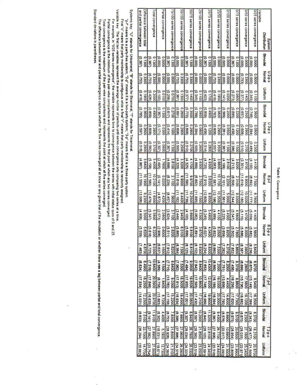
39