Family Migration and Labor Market Outcomes

Transcription

1 Family Migration and Labor Market Outcomes (JOB MARKET PAPER) Ahu Gemici University of Pennsylvania January 2006 I am truly indebted to Kenneth Wolpin, Antonio Merlo and Petra Todd for their generous support and encouragement. I also benefited from conversations with Nicola Persico, John Knowles, Aureo De Paula, Phillip Kircher, Kurtulus Gemici, Manolis Galenianos, Melissa Tartari, Guido Menzio, Jorge R. Gallardo-Garcia and Limor Golan.

2 Abstract Job search and migration behavior of married couples differ markedly from that of singles, which suggests that marriage, migration and labor market decisions are interrelated. Interregional moves are associated with higher wages for married men, single men, and single women, but married women do not realize much wage growth through migration and, in fact, are less likely to be employed following a move. The goal of this paper is to assess the implications of joint geographic location constraints on the migration patterns, labor market outcomes and marital stability of men and women. I develop a model of household migration decisions in a dynamic framework with intra-household bargaining and estimate it using data from the Panel Study of Income Dynamics (PSID). The results show that marriage involves compromises for both spouses in terms of foregone job opportunities. However, migration decisions occur more often in response to men s opportunities, in part because women have lower wage offers, a lower arrival rate of offers, and a lower variance in offers. Married women expect migration-induced interruptions in their employment spells, which makes them willing to accept lower wages. When acting as single agents or when there are no geographic location constraints, the accepted wages of both men and women increase considerably. I also find that the possibility of divorce is an important factor in household mobility, as spouses are less willing to make compromises when faced with the possibility of future separation. JEL Classification Code: J12, J16, J31, J61 Keywords: Family Migration, Gender Wage Gap, Household Labor Supply

3 1 Introduction Joint migration decisions have become increasingly relevant in the modern labor market with the rising labor force attachment of women. Spousal considerations are important determinants of male and female job search behavior and choice of location. 1 This paper theoretically and empirically analyzes the relation between marriage, migration and labor supply decisions. Evidence from the Panel Study of Income Dynamics shows that the relationship between migration and wage/employment outcomes of men and women significantly differs by marital status. Figure 1 shows that married men who move at least once during the course of their marriage have on average higher wages than those who never move. 2 For married women, however, there is no significant difference by migrant status. As seen in Table 1, married women are also less likely to remain employed following a move. These gender differences are not observed for single men and women, for whom migration is associated with higher wages and for whom the likelihood of remaining employed following a move is similar. This paper addresses three main questions: (1) What accounts for the observed relationship between migration and labor market outcomes of married men and women? (2) What are the migration responses of married people to differences in wage opportunities across locations and (3) To what extent do family migration decisions contribute to the observed gender wage gap? In particular, if married individuals move in response to their spouses job opportunities as well as their own, then their labor market decisions can be markedly different than that of single individuals. The implications of joint location constraints on the observed wage and employment outcomes of married couples can only be discerned after taking the selective nature of migration and joint job search behavior into account. To address the questions of interest, I develop and estimate a dynamic model of married couples decisions regarding geographic location and employment status in a framework with intra-household bargaining. 1 The early literature on migration recognized the role of the family in location and labor supply decisions (Mincer (1978), Frank (1978)). I briefly summarize this literature in Section 2. 2 A location is defined as a Census Division in the United States. Census divisions are groupings of states that have been defined by the U.S. Census Bureau for the purpose of data presentation. There are nine census divisions in the United States. See Appendix for a map and a list of the Census divisions. 1

4 In my model, each year a married couple makes decisions about whether (1) they will stay in their current location or move to a different location, (2) whether the husband will work, (3) whether the wife will work, (4) whether they will remain married. The spouses respective shares of the total household utility are determined in a Nash bargaining framework with the threat point specified as the value of divorce. Upon divorce, individuals continue to make employment and migration decisions as single agents. The household chooses among multiple locations that differ in terms of their wage offer distributions and non-pecuniary benefits. In addition to location, the wage offer distributions differ by gender, education and labor market experience, which accumulates endogenously. Men and women are allowed to differ in their preferences for leisure. I structurally estimate the model using data from the Panel Study of Income Dynamics, which has detailed information on employment, wage and location histories of married couples between the years 1968 and The model is estimated by simulated method of moments, which minimizes a weighted average distance between a set of sample moments and moments simulated from the model (McFadden (1989)). In this paper, I show that a unitary and static approach to the household s problem will fail to account for important aspects of the joint location and labor supply problem of married couples. 3 The point of departure is the incorporation of the household s decision problem in a dynamic search environment with uncertainty, allowing for differences in wage offer distributions across locations as well as between men and women, with intra-household bargaining, endogenous experience accumulation and the possibility of divorce. This framework allows for a rich representation of the tradeoffs that a couple faces in making employment and migration decisions. Such a representation can provide important insights into how the family members joint location constraint affects their labor market decisions. First, this constraint leads to both spouses making compromises in terms of their labor market opportunities. Family members do not always accept the best offers they have from other locations, because the costs and gains 3 By static I refer to the type of models that do not incorporate uncertainty in future wage opportunities or in preferences. 2

5 from relocation are also influenced by the expected value of search of their partner in the new location. Household bargaining provides the mechanism by which such costs or gains from relocation (or no relocation) are shared. However, when the costs that one spouse incurs are too high relative to the gains from marriage or his/her partner s gains from relocation, it is optimal for the couple to divorce. In contrast, in cases where there are gains to remaining married, an individual might reject a high wage offer because his/her spouse does not face a favorable labor market environment in the new location. Therefore, in addition to current wage offers, the expected value of search of the partners across locations as well as the expected value of remaining married are important determinants of married couples location decisions. Second, the possibility of divorce can be an important factor in migration and labor market decisions of the couples. In the model, family members accumulate work experience endogenously. Faced with the possibility of divorce, family members are more reluctant to choose migrationinduced disruptions to their employment spells because it adversely affects their future value of being single. In this case, the cost to relocation for the trailer spouse will include his/her lower future wage offers due to lower accumulated work experience. 4 The incentives to incur or share such costs are diminished given the possibility of divorce. The estimated model is used to perform four counterfactual experiments to quantify the implications of joint location constraints on the migration patterns and labor market outcomes of married men and women. The first examines the extent to which joint decision making within the household contributes to the observed location and employment outcomes of married men and women. Specifically, I simulate the behavior of all individuals were they single instead of married. I find that as singles, men move more frequently. Married men forego some job opportunities due to the presence of their wives, whereas when single, they do not. As singles, women s moving rates are lower compared to when they are married. 5 In the absence of a spouse who often initiates moves, women have a lower propensity to migrate, because women face less 4 Lundberg and Pollak (2001) use the term trailer spouse to denote the family member that moves together with his/her spouse who has a job offer from another location 5 My findings about the effect of family ties on migration are consistent with Mincer (1978) s conjecture that married men are tied stayers and married women are tied movers. 3

6 variation in their wage offers across locations. This result shows that for married couples, the household moves are generally initiated by the husband. I find that average male accepted wages increase by 24 percent and female accepted wages increase by 14 percent under the singles scenario. Male accepted wages increase, mainly due to their higher mobility rates. When single, males are able to take full advantage of their different job opportunities across locations. Accepted wages of women as single agents are higher for two reasons. First, when single, women only move for their own employment opportunities. Second, in the absence of migration-induced interruptions in their employment spells, women are willing to wait longer for high wage offers. This is because returns to higher wage jobs increase due to longer expected employment spells. Under the second counterfactual, I eliminate the possibility of moving in order to examine how mobility concerns contribute to labor market decisions of married couples. 6 I find that with no possibility of moving the female-to-male employment ratio increases from 0.58 to Moreover, the gender wage gap decreases: The female-to-male accepted wage ratio is 0.68 for the baseline, in comparison with 0.75 with no possibility of moving. When there is no migration, women work more and accept higher wages. This is because women expect fewer interruptions in their employment spells, which leads to higher returns to accumulated work experience and higher reservation wages compared to the baseline. Under the third counterfactual, I change the mean wage offers of locations to quantify the migration responses of married couples to changes in their wage opportunities across locations. I find that the extent to which the migration rates of males increase in response to changes in their wage offer distributions strongly depends on their wives wage prospects across locations. Under the fourth counterfactual, I equate the wage offer distributions of men and women. I find that when they face equal wage offer distributions, migration occurs in response to the job opportunities of both spouses. Therefore, when there are no differences in the labor market opportunities they face across locations, migration is associated with higher wages for women as 6 In this counterfactual I let the agents face a national wage offer distribution with no geographic location constraints. 4

7 well as men. In the baseline case, the percentage difference between the wages of women who move and those who never move is -1.0 percent. With equal wage offer distributions to that of men, women experience an 18 percent wage growth when they move. The paper is organized as follows. Section 2 discusses the related literature. Section 3 describes the structure of the model. Section 4 outlines the numerical solution algorithm. Section 5 presents the data. Section 6 gives the estimation method and estimation results. Section 7 outlines the results from the counterfactual experiments. Section 8 concludes. 2 Related Literature The migration literature in economics can be classified into two groups of studies. The first group consists of studies that analyze migration at the individual level, where the main focus is on the determinants of moving decisions and the returns to migration in terms of lifetime wages and earnings. Most of these studies analyze migration with a perfect foresight setting without uncertainty about future employment and earnings. One paper that incorporates individual migration in a dynamic setting with uncertainty is Kennan and Walker (2006), which develops a structural dynamic migration model and estimates it using panel data from the NLSY. Kennan and Walker find that individuals migration decisions are significantly influenced by their income prospects in different locations. My paper is most closely related to Kennan and Walker (2006) in terms of general approach, but I extend their paper to incorporate family migration decisions, rather than individual decisions. The second group of studies analyze migration at the household level. One of the earliest papers to emphasize the importance of studying migration as a family decision is Mincer (1978). 7 Mincer (1978) presents a model where families make migration decisions based on a one time comparison of total gains and/or losses of the spouses earnings. Mincer (1978) introduces the 7 This paper is also similar to a number of studies that have explored household search in the labor market. Dey and Flinn (2005) look at the relationship between health insurance coverage and wage and employment outcomes at a household level. I focus on migration decisions in addition to labor market decisions of the household. I also extend these studies to account for the strategic interactions between the spouses. 5

8 idea that family mobility decisions might play a reinforcing role in the observed differences between men and women in terms of their labor market outcomes. These ideas are also explored by Frank (1978), who develops a model of joint placement where families maximize total income by choosing a work location within a two-period setting. He uses this model to quantify the fraction of the unexplained wage gap that results from family migration. This paper extends these earlier ideas and analyses in the following ways. First, it incorporates household migration decisions between multiple locations in a dynamic setting with uncertainty and the possibility of making multiple moves. The sources of uncertainty are future job opportunities in different locations as well as the possibility of divorce. Moreover, family members accumulate experience while working. With a future possibility of divorce, family members are therefore more reluctant to choose migration-induced interruptions to their employment spells. In short, the dynamic framework together with a non-unitary approach to the household problem allow for a richer representation of the family s decision-making. Second, the model distinguishes between accepted and offered wage distributions of men and women, which is important for the purposes of understanding the sources of gender wage differences. My results support Mincer s conjecture that family mobility concerns magnify gender wage gaps. Family migration has also been explored by Costa and Kahn (2000) and Compton and Pollak (2004), with a focus on the impact of the changing migration patterns of married couples on the composition of educational attainment in large metropolitan areas in the US. These two papers explore the reasons behind the increased concentration of so-called power couples, couples in which both spouses have college degrees, in large metropolitan areas. In relation to these studies, this paper could be viewed as providing insight into the mechanism underlying joint migration decisions of educated couples. Family migration decisions within a intra-household bargaining framework has also been studied by Lundberg and Pollak (2001). They use a two-stage model of family location decisions to illustrate how inefficiencies may arise if current decisions have implications for future bargaining power of the family members. They show that under lack of commitment, family mi- 6

9 gration decisions give rise to inefficiencies. This paper extends their study by incorporating job search, endogenous experience accumulation and uncertainty in the intra-household bargaining framework. 3 Model I model the decision of married couples starting from the time of marriage and the time horizon is 30 periods. Each period, the individuals make decisions regarding their location, labor supply and marital status. In other words, each period the couple makes decisions about whether they will stay in their current location or move to a different location, whether the husband will work, whether the wife will work, and whether they will remain married. A period corresponds to a calendar year. A location corresponds to one of the 9 Census Divisions in the United States. 8 The household can choose between current and one alternative location, chosen at random. In what follows, I label the current location by A and one of the 8 other possible locations as B. Each period, the couple can either stay in their current location A, or move to one other candidate location B. The candidate location B is chosen from the other 8 possible locations at random. The probability of having the opportunity to move to location B is assumed to be different if B is the home location of the couple. I define the home location of the family as the place where the husband grew up. 9 If the couple is already in their home location, the probability of having the opportunity to move to location B is simply 1 8 for each of the 8 possible locations. On the other hand, if they are not in their home location (i.e., if home is one of the 8 other locations), the probability of having the opportunity to move to location B is given as data. 8 A list of the Census Divisions together with a map can be found in Appendix A. 9 I disregard the home location of the wife mainly because this information is not available in the PSID 7

10 follows, pr(b) = p home if B=home 1 p home 7 if B home Job offers of the husband and wife arrive from the two possible locations (current and candidate) with a certain probability. The probability that an agent gets an offer from the candidate location is independent of offers to him/her from the current location and it depends on the agent s employment status and education. The probabilities that each spouse gets an offer are also independent of each other. In other words, job offers may arrive from the two possible locations (current and candidate) to both spouses, one of the spouses, or neither of them. When employed, the agents continue to get offers on-the-job at a potentially different frequency relative to when they are not working. The probability of receiving a job offer from location B while the agent is in location A is given by λ i (g,e;a,b,h), where g, e and H denote the education level, current employment status, and the home location of the agent. 10 The wage offers are drawn from a distribution that depends on the characteristics of the individuals and they are allowed to differ by sex and location. The wage offer of individual i (i = h for husband, and i = w for wife) from location k is given by, ln ω i,k = α 0,i,k + α 1 g i + α 2 x i + α 3 x i 2 + ν i,k i = h,w k = 1,2,..,9 where x i denotes the work experience of spouse i. The coefficients α 1,α 2,α 3 are assumed to be the same between men and women. The joint distribution of ν k = (ν h,k,ν w,k ) is assumed to be normal so that ν k N(0,Σ) for each k. This random component of the wage draws is assumed be independent across locations. 10 The education variable corresponds to whether the individual has a college degree or not. 8

11 3.1 Preferences Individuals derive utility from marriage (M), from leisure if not working (b), and they derive utility from residing in a certain location (π k ). The location utilities (π k ), which are allowed to differ by location, can be thought of as amenity values or other forms of non-pecuniary benefits. Also, individuals derive an extra utility from residing in their home location H. I allow for a psychic cost (ψ) associated with changing locations. An interpretation of this moving cost is that people may be reluctant to leave the environment they are familiar with. I allow this utility cost to depend on the individual s employment status, whether there are any children in the household, on the number of periods the couple has resided in their current location and a stochastic component which is drawn every period. The cost of moving from location l to location k is given as follows: ψ i (n,e i, 1,d l ;l,k) = γ 1 1{n = 1} + γ 2 e i, 1 + γ 3 d l + ε 1,i, i = h,w where n indicates whether the couple has any children, e i, 1 denotes the employment status of the individual i in the previous period, and d l is the number of periods the couple has resided in location l. Agents get utility from not working. This utility is a function of whether the couple has any children and the effect of children on the value of leisure is allowed to differ by gender so that the utility from not working is given as: b i (n) = γ 4,i 1{n = 1} + ε 2,i, i = h,w ε 2,i N(0,σ 2 ) Each period, the couple gets a marriage bonus that depends on the duration of marriage (d M ) and a stochastic shock. This marriage bonus is assumed to be the same for the husband and the 9

12 wife and is given by: M(d M ) = γ 5 + γ 6 d M + ε 3 ε 3 N(0,σ 3 ) Last, the location utility of individual i whose home location is H and who is in location k is: π(g;k,h) = η(g;k) + γ 7 1{k = H} where η(g; k) denotes the nonpecuniary benefits for each location that differs by whether the individual has a college degree or not. Given the above, the utility of an agent at period t whose location in the previous period and current period is l and k, respectively, is given by: u i = ψ i (n,e i, 1,d l ;l,k) 1{l k} + b i (n) + M(d M ) + π(g;k,h) i = h,w 3.2 State Space Initial conditions of a married couple at the time of marriage (t = 1) are their starting location (l(0)), their employment status in the previous period (e h (0),e w (0)), their wages if they were working in the previous period (ν h (0),ν w (0)), total labor market experience (x h (0),x w (0)), home location (H) and education (g h,g w ). Duration at location is assumed to be 0 at the start of the marriage. 11 The couple s state space at time t > 1 is: Ω i (t) = l(t 1),e h (t 1),e w (t 1),ν h (t 1),ν w (t 1), x h (t),x w (t),n(t),d l (t),d M (t),h,g h,g w, ε 1,h (t),ε 1,h (t),ε 2,h (t),ε 2,w (t),ε 3 (t),ν h (t),ν w (t) 11 I define the duration at location as the number of periods the couple has resided in a particular location since the start of the marriage. 10

13 Total labor market experience of the individual in t+1 is determined by his/her work experience, x i (t), and employment choice e i (t) in period t: x i (t) if e i (t) = 0 x i (t + 1) = x i (t) + 1 if e i (t) = 1 Also, the number of periods the couple has resided in a location is determined by the past duration at that location and the couple s moving choice in period t. If the couple changed locations in the previous period, their duration at location is set to 0 so that the duration at location is given as follows: d k (t) + 1 if k(t) = l(t) d k (t + 1) = 0 if k(t) l(t) If the couple remains married, the duration of marriage, d M (t + 1), is determined as follows: d M (t + 1) = d M (t) + 1 Fertility is exogenous so that in each period the wife gives birth with a certain probability: n(t + 1) = n(t) if n(t) = 1 1 with probability p n if n(t) = 0 0 with probability 1 p n if n(t) = Problem of the Household Each period, the couple makes decisions about whether they will stay in their current location or move to a different location, whether the husband will work, whether the wife will work and whether they will remain married. For each location/employment alternative, they determine 11

14 their respective shares of the total household utility as the solution to a symmetric Nash bargaining problem. The threat point in their problem is specified as the value of divorce, which is the discounted sum of future utilities that the spouses would obtain as single agents. The set of alternatives that are available to the agents are different depending on their job offers from location A and location B. For example, suppose a couple at period t, is currently working in location A at wages (ω h,ω w ). Also, suppose that this couple gets offers from location A and location B, given by ( ω A h, ωa w) and ( ω B h, ωb w). The set of alternatives available to this couple are as follows: (1) Stay/Both continue to work at (ω h,ω w ), (2) Stay/Both work at ( ω A h,ωa w), (3) Stay/Both work at (ω A h, ωa w), (4) Stay/Both work at ( ω A h, ωa w), (5) Stay/Only Husband work at current wage or (6) his new wage, (7) Stay/Only Wife work at current wage or (8) her new wage, (9) Stay/Neither work, (10) Move/Both work at ( ω h B, ωb w ), (11) Move/Only husband work at ω h B, (12) Move/Only wife work at ωb w, (13) Move/Neither work, (14) Divorce and the spouses stay or move alone. The symmetric Nash bargaining solution implies that conditional on each alternative J (where J=1,..,14), each spouse gets half of the total marriage surplus, so that spouse i gets, u i (t J) + Γ i (t J) + βev i (Ω(t + 1) J) = V i (t) + 1 ω h (t) + ω w (t) + u h (t J) + u w (t J)+ 2 βev h (Ω(t + 1) J) + βev w (Ω(t + 1) J) V h (t) V w (t) Γ i (t J) denotes the intra-household utility transfer that spouse i gets conditional on alternative J. The couple chooses the alternative that maximizes their expected present lifetime utility so that their value function can be written as follows: V i (t) = max {u i(t J) + Γ i (t J) + βev i (Ω(t + 1) J)} J {1,..,14} V i (t) denotes the outside option of spouse i. It is the maximum over alternative-specific value functions associated with being a single agent. Given the wage offers described above, the alternatives available to a single agent are: (1) Stay and continue to work at ω A i, (2) Stay and accept new offer ω A i, (3) Stay and don t work, (4) Move and work at ωb i, (5) Move and don t 12

15 work. Then, V i (t) is given as follows: V i (t) = max {ū i(t J) + βe V i (Ω(t + 1) J)} J {1,..,5} It can be seen in Figure E that the couple s different location and employment options correspond to different utility possibility frontiers. The couple chooses the alternative that corresponds to the outermost utility possibility frontier. Figure E shows the case where moving and both working at their offered wages at location B is preferred to staying and both continuing to work at their current wages at location A. Vh and V w are the best available outside options of the husband and wife. As long as there exists some agreement preferred by both parties to the disagreement outcome, the couple will stay married and choose the alternative with the highest surplus. Figure F shows the case where the household chooses to divorce. In this example, the alternative that is associated with the highest utility possibility frontier is {Move}, but the outside options of the husband and wife give higher utility. Figure E: Decision of the Household V h UPF Move UPF Stay V h V w V w The factors that influence the household s employment and migration decisions are as follows. Suppose the couple is in location A and both the husband and wife are working in their current location. For simplicity, suppose that the offer situation of the couple is such that only one of the 13

16 Figure F: Decision of the Household V h V h V w UPF Move UPF Stay spouses gets a job offer from location B and neither gets a job offer from their current location. Following the language of Lundberg and Pollak (2001), I will denote the spouse that gets an offer from location B as the leading spouse and the spouse who does not get an offer as the trailer spouse. The value of moving to location B with the leading spouse working at the offered wage and the trailer spouse searching is determined by the following factors: V w 1. Trailer spouse s value of search in location B which is determined by location B s wage offer distribution, the utility from staying at home for the trailer spouse, and his/her job offer arrival rates. The value of search differs across locations mainly because the arrival rate of offers from a certain location vary according to whether the individual resides in that location or not. 2. Leading spouse s value of on-the-job search in location B which is determined by his/her location B wage offer distribution and job offer arrival rates while working. 3. Non-pecuniary benefits of location B and whether location B is their home location. 4. Moving costs which is determined by the couple s joint employment status, whether they 14

17 have any children and how long they have been residing in location A. 5. Outside options of the spouses. The tradeoff for the trailer spouse is as follows. If he/she moves, then he/she will not be receiving earnings that period but will get utility from staying at home. The dynamic component of the trade-off for the trailer spouse is that not working this period means less human capital accumulation and hence lower wage offers in the future. Utility is transferrable between the spouses, which implies that the trailer spouse can be compensated for foregone earnings and lower accumulation of work experience. 4 Solution Method Given the above formulation, we can solve the problem recursively, starting from period T = 30. At period 30, the value functions are the current returns to choosing each alternative. We can calculate these alternative-specific value functions for every element of the state space at period T and then calculate the maximum for each element in the state space, and integrate over the shocks. In this way, we will obtain the expected value of the maximum alternative-specific value function for each element in the state space at period T, E T [max{v h (Ω(T) d(t) = 1),...,V h (Ω(T) d(t) = 9)} Ω(T)] E T [max{v w (Ω(T) d(t) = 1),...,V w (Ω(T) d(t) = 9)} Ω(T)] Given these above Emax functions, we can calculate V h (T 1) and V w (T 1) for all possible state space elements in period T 1 (all possible points in Ω(T 1)). The value functions of males and females can be calculated at each period using this backwards recursion method. Calculation of the Emax functions at each point in the state space creates a computational difficulty. I circumvent this problem by calculating the Emax values at a subset of the state space and using the interpolation method proposed by Keane and Wolpin (1994). 15

18 5 Data The core PSID sample consists of two independent samples: a cross-sectional national sample, known as the SRC (Survey Research Center) sample, and a national sample of low-income families, known as the SEO (Survey of Economics Opportunities) sample. This core sample originated in 1968 and the individuals from families in the core sample were interviewed from 1968 to 1996 every year. In 1990 and 1997, a supplemental sample of Latino households and Immigrant families were added to the core PSID sample. My estimation sample only includes those individuals who are associated with families from the SRC. The criteria that I use to construct the estimation sample are as follows. I follow males from the time of their marriage through the time of their divorce, their last interview or until they are age 50, depending on which event occurs first. The estimation sample includes white males and females who marry only once during the time frame that I observe them and for whom the age of marriage is above 18 or below percent of the sample consists of males who got married before age 25. I exclude those males who are observed for only less than three periods. There are 1499 males in the sample. I follow the employment, wage and location histories of these male heads and their wives during the course of their marriage. The PSID collects retrospective histories of marriages for those individuals who are of marriageeligible age and who are living in a PSID family at the time of the interview in the waves. The variable for the year of marriage is only available for such individuals. For those who are out of the sample by 1985, I assume that the time of marriage is the first year that I start observing them to be married. I consider an individual to be married if the marital status of the head at the time of interview is Married or permanently cohabiting. Divorce is assumed to occur when the individual is observed to be married in period t and not married in the next period. A location is defined as a Census Division. Census divisions are groupings of states that have been defined by the U.S. Census Bureau for the purpose of data presentation. There are nine census divisions in the United States: New England, Middle Atlantic, East North Central, West 16

19 North Central, South Atlantic, East South Central, West South Central, Mountain, Pacific. The list of states that are included in each division and a map of the census divisions are included in the Appendix. A couple is considered to have relocated if their location in period t is different from their location in the next period. During the course of the year, the couples are assumed to remain in the same location. PSID has detailed information on employment, earnings and total labor market experience of household heads and wives. I obtain the employment status of the individuals through the number of hours they work during the year. I consider an individual to be working if their hours of work exceeds 1000 hours for a given year. The annual earnings is computed by multiplying their hourly wages by 2000 (50 weeks X 40 hrs/wk) hours so that the variation in earnings only reflects variation in the hourly wages. I construct the labor market experience variable of the household head and wife as follows. The PSID has information on the amount of time the household head and wife has worked since the age of 18 until the time of interview. The work experience variable is self-reported and the question is asked of only new heads or wives in the household. The question is asked to all heads and wives for only certain years. For each individual, I take the value of the work experience variable that is reported in the years that they are asked and work either backwards or forwards taking into account the employment status for each preceding or subsequent year. I consider the work experience of an individual to be 0 at age 18. For such individuals, I update the experience variable according to their subsequent employment status during the time that I observe them. 5.1 Descriptive Statistics Table 2 displays the basic descriptive statistics for the estimation sample. The average length of time that a couple is observed in the sample is years. The average age of marriage for the males in the sample is and it is for the females. The proportion of those couples where both the husband and wife are college educated is percent percent of couples are those with only one spouse college educated and percent are couples with no college 17

20 education. The average total labor market experience of the males at the time of marriage is approximately 6.55 years and for the females it is 4.06 years. Table 2 also shows the moving rates. Approximately 19 percent of the couples in the sample are observed to change locations at least once. Of all the moves that I observe for the people in the sample, approximately 30 percent are moves that are back to the home location of the couple. I define the home location as the place where the head grew up. The distribution of the couples by division in the fist period is displayed in Table 3. Table 4 shows the in-migration and out-migration rates for each Census region. 12 In-migration is defined as migration into an area during a given period and out-migration is defined as migration out of an area during a given period. These rates are given as the number of in-migrants and outmigrants as a proportion of the total number of couples in that area. An interesting aspect of the domestic migration patterns is that the location with the highest in-migration rate is also the location with the highest out-migration rate. The same holds for the location with the lowest in- and out-migration rate. The highest levels of both in- and out-migration occurs in the South and West regions and the lowest levels occur in the Northeast region. Table 5 shows the annual wages of males and females by each of the 9 Census Divisions. It can be seen that men and women differ in terms of the rankings of their mean accepted wages across locations. For example, for college educated men, the highest accepted mean wages are observed in the East North Central divisions. On the other hand, for college educated women, the highest mean wages are observed in the Middle Atlantic division. The per-period (annual) moving rates by the characteristics of the couples in the sample are as follows. Figure 2 shows that the migration rates decrease by the number of periods a couple has resided in a certain location. Table 6 shows migration rates by the joint education level, joint employment status of the couples as well as by whether they have any children. Couples are classified according to their joint education level as follows: (1) Both spouses are college 12 Census Regions are groups of Census Divisions. The in- and out-migration rates are reported by regions only. I do not disaggregate further (for example into Census divisions), due to low migration rates. A list of the Census Regions can be found in the Appendix. 18

21 educated, (2) Only husband is college educated, (3) Only wife is college educated, (4) Neither is college educated. Also, couples are classified according to their joint employment status as follows: (1) Both spouses are working, (2) Only husband is working, (3) Only wife is working, (4) Neither spouse is working. The couples are least likely to move when both spouses are working in their current location. Table 6 shows that 1.71 percent of couples with both spouses working migrate whereas for couples with neither spouse working, the migration rate is 4.07 percent. Table 6 also shows that couples in which both spouses are college-educated are the ones most likely to move and couples in which neither spouse is college-educated are the ones least likely to move. The migration rate of couples in which only the husband is college educated is similar to the migration rates of couples in which both spouses are college educated. On the other hand, the migration rate of couples in which only the wife is college-educated is similar to couples with no college education. This suggests that it is the husband s education level that matters for the migration patterns of couples and not the wife s education level. 13 Also, couples with children are less likely to change locations than the couples who do not have children. For couples with children, the migration rate is 4.00 percent whereas for couples with no children the migration rate is 2.15 percent. Tables 7-8 and Figure 3-4 display the labor market outcomes of the couples by their migrant status and their education level. Here I look at two different aspects of the data: (1) Transition rates between employment states for men and women in periods of relocation and periods of no relocation, (2) Wages of men and women by whether they ever relocated during the course of their marriage. Tables 7 and 8 show the employment rates of men and women conditional on their employment status in the preceding period, making a distinction between whether they relocated or not. Conditional on not working in period t, males are three times more likely to become employed in period t + 1 in periods where they do not move: Proportion of those who become employed is percent for males and percent for females. On the other hand if they move, males are approximately seven times more likely to become employed relative to their wives: The 13 Costa and Kahn (2000) also finds this pattern by education. 19

22 proportion of those who become employed in a different location is 3.37 percent for males and 0.52 percent for the females. Also, females are more likely to remain unemployed when they move in comparison to when they stay. These transition rates show that the proportion of men who continue working (or start working) in their new location is higher than that of women. Relocation is associated with lower employment rates for women (in comparison to the periods where they remain in the same location). This is not the case for men. Lastly, looking at the males and females in the sample by whether they ever moved during the course of their marriage or not reveals that there is a strong relationship between migration and the labor market outcomes of married people. Figure 3 shows the wages of men by their total labor market experience, education and moving status. For college educated married men, those who moved at least once have higher wages. For married men who do not have a college degree, those who moved at least once have similar wages to those who never move. Figure 4 shows the wages of working women by their total labor market experience, education and moving status. For college educated married women, migration is associated with lower wages. In other words, those college educated women who moved at least once have lower wages than those who never moved during the course of their marriage. On the other hand, for married women who are not college educated, the wages of those that have moved at least once and those that have never moved are similar. 6 Estimation Results Estimation is by simulated method of moments where the model parameters are chosen to minimize a weighted average distance between a set of sample moments and moments simulated from the model. The weights are the inverse of the estimated variances of the sample moments. The moments used in the estimation that are related to the employment rates and accepted wages are as follows: 1. Proportion of husbands and wives who work by work experience, education level and 20

23 whether they have children. 2. Proportion of husbands and wives who work by location and education level. 3. Proportion of husbands and wives by the education level of their spouse. 4. Accepted wages of husbands and wives who work by work experience, education level and whether they have children. 5. Accepted wages of husbands and wives who work by location and education level. 6. Accepted wages of husbands and wives by the education level of their spouse. 7. Accepted wages of husbands and wives by work experience and by moving status Proportion of husbands and wives who work in a given period by whether they were working in a preceding period and whether they changed their location between the two consecutive periods. 9. Log wage difference of the husbands and wives by whether they moved since the preceding period. 10. Standard deviation of the accepted wages and the correlation between the wages of husbands and wives. Moments related to the migration rates are given as follows: 1. Proportion of couples who move by age of head, location tenure, joint employment status, joint education level and whether the couple has any children. 2. In- and out-migration rates for each Census division. 3. Divorce Rates by duration of marriage and moving status. 4. Transition rates between Census regions. 14 The moving status refers to whether the couple has ever changed location during the course of their marriage. 21

24 5. Proportion of moves that are back to home location. 6.1 Model Fit Figures 5-12 and Tables 9-15 show the model fit for chosen moments of the estimation. The model predictions in general do well in comparison to the data moments. Figures 5-10 show that the model does a good job in fitting the wage and employment profiles of men and women by their location, education and years of work experience. The model captures the variation in male and female accepted wages across locations and across education groups. In particular, Figures 11 and 12 show that the model captures the fact that migration is associated with higher wages for married men, but not for married women. Table 9 shows that the model captures the fact that in comparison to married women, married men are more likely to remain employed following a move. The model fit for the unconditional transition rates between employment status and location between two consecutive periods are presented in Tables 10 and 11. As in the data, the model predicts that men are much more likely to change locations and become employed compared to women. For example, conditional on not working in the current location, 2.06 percent of married men change locations and become employed at the destination location. On the other hand, this percentage is only 0.88 for married women. Table 12 shows the moments related to the moving rates and divorce rates for the data and simulations. In the data, 19 percent of couples move at least once during the course of their marriage, and in the simulations this ratio is 21 percent. Also, in the data, 21 percent of couples divorce and in the simulations this ratio is 18 percent. The model simulations also capture the patterns of moving rates by the age of head. Table 14 shows that the model captures the fact that moving rates decrease by the age of head. The transition matrix by region, in the data and the model simulations is displayed in Table 15. This table presents the proportion of couples who move to region j, conditional on being in region i for all regions. 15 It can be seen that the 15 The transition matrix aggregates divisions into regions. A list of which divisions are included in each region is provided in the Appendix. This aggregation is mainly due to the small number of moves in each cell when we look at the transition rates between each division. 22

25 model simulations provide a reasonable fit to the transition rates in the data, except for the fact that the model overstates the number of moves that are to the Northeast region. 6.2 Parameter Estimates Tables 16 through 20 report the parameter estimates. Table 16 displays the utility function parameter estimates for males and females. It can be seen that the value attached to not working is considerably different between men and women. I allow this utility to depend on whether the family has any children or not. The estimated value of leisure parameter estimates are such that the value of not working for men and women with kids is on average $4,159 (=$3,205+$954) and $11,438 (=$8,603+$2,835), respectively. 16 Also, the value of not working for men and women without children is on average $3,205 and $8,603, respectively. Table 19 displays the wage offer function parameter estimates for men and women. The education and experience effect on wage offers are assumed to be the same for men and women. The constant component of the wage offers are allowed to differ by sex as well as by geographic location. It can be seen in Table 19 that men and women s mean wage offers (for 0 experience level and no college education) differ considerably across locations. For example, while the West North Central division has the highest mean wage offers for women compared to the other locations, it has one of the lower mean wage offers for men. Moreover, the variation across locations in terms of mean wage offers is higher for men compared to women: The standard deviation of mean wage offers given 0 experience level and no college education is $1,577 for men and $1,213 for women. Table 18 displays the parameter estimates for the non-pecuniary benefits for each location. This is the utility that the agents get from being in a certain location in each period. I allow this utility to depend on whether the agents have a college degree or not. The value for the non-pecuniary benefits of one of the locations is normalized to 0 within each education group. The estimates show that there is a large variation in the non-pecuniary benefits across locations 16 The utilities of not working can be expressed in monetary equivalent terms due to the linearity of the utility function 23

26 for both educated and uneducated individuals. Moreover, the parameter estimates show that the ranking of locations in terms of their non-pecuniary benefits is different between the two education groups. For example, the Pacific division is the location that offers the highest nonpecuniary benefits for college educated individuals, while it is the place with the lowest nonpecuniary benefits for the individuals with no college education. This is consistent with the fact that the Pacific division has low mean accepted wages for educated individuals (compared to the mean accepted wages for educated people in other locations) and high mean accepted wages for the uneducated group. Individuals have higher reservation wages to move to locations with low non-pecuniary benefits, and therefore the model predicts a negative correlation between the non-pecuniary benefits in a location and the mean accepted wages. This can be seen in Table 21 which shows the Spearman rank-order correlation coefficient for the non-pecuniary benefits and the accepted wages for each location by the different education groups. It can be seen that the model predicts a negative and large correlation coefficient between the non-pecuniary benefits and the accepted wages within each education group. Moreover, the correlation between the non-pecuniary benefits across locations and accepted wages is considerably higher for husbands compared to wives, for those who are not college educated. On the other hand, the correlation is considerably higher for the wives for the educated group. This is due to the fact that when the wives are not college educated, the destination location is generally determined by the husband s opportunities. However, when the wives are college educated so that they have relatively more equal labor market opportunities compared to that of the husbands, the destinations are also determined by the wife s wage opportunities. Table 20 reports the estimates for the parameters related to the probability of getting job offers. I allow these offer probabilities to differ by sex, education and current employment status. The parameter estimates show that the arrival rates of job offers differ considerably by gender, employment status and education level. They also differ considerably by whether the job offer is from current location of residence or a different location. For a male who is not working, and college educated, the arrival rate of a job offer from his current location is 0.66 while it is

27 for the female. For a male who is not working, and not college educated, the arrival rate of a job offer from his current location is 0.64 while it is 0.34 for the female. For both education groups, males receive job offers from current location at a lower rate if they are working compared to when they are not working (0.29 if college educated and 0.11 if not). The job offer arrival rate for unemployed college educated women is considerably lower than that of unemployed women with no college education (0.03 and 0.34, respectively). This is due to the fact that the transition rate from unemployment to employment is similar for college and non-college women, despite the fact that college educated women have a higher opportunity cost of not working. In comparison, the job offer arrival rate for employed college educated women is considerably lower than that of employed women with no college education (0.39 and 0.00, respectively). College educated women are more willing to incur wage losses following a move, mainly due to the fact that they will continue to get job offers at a high arrival rate at the destination location. On the other hand, this is not true for women who are not educated, mainly because their arrival rate of job offers from current location is very low. Therefore, they are less willing to incur wage losses when they move to a destination location. The model captures this fact through their different arrival rate of job offers. Lastly, the parameter estimates show that men overall have higher arrival rates of offers compared to women. 7 Counterfactual Experiments The goal of this paper is to determine to what extent location constraints that married couples face in the labor market affect their migration patterns, wage and employment outcomes. To address this question, the model is simulated under a number of counterfactual scenarios. These counterfactuals are as follows: (1) Simulate behavior for single men and women by making the couples divorce in the first year of their marriage, (2) Eliminate the possibility of moving, (3) Change the mean wage offers across locations, (4) Equate wage offer distributions of men and women. 25

28 7.1 Counterfactual 1: Divorce in Period 1 Under the first counterfactual scenario, I make the couples divorce before the first year of their marriage. The outcomes of interest are the migration rates, wage and employment profiles of men and women as single agents. This counterfactual examines the extent to which joint decision making within the household contributes to the observed migration patterns and differences in the gender differences in wage and employment profiles. I assume that the divorce before the first year of marriage comes as a surprise to the agents, and therefore assume that their initial conditions at the age of marriage do not change. The men and women under the counterfactual scenario have the same characteristics, and face the same environment as the baseline. In particular, they face the same probability of having children. This is to abstract from children in this counterfactual experiment. The parameter estimates show that especially the wives get high utility of leisure when there are children present. When single, I allow them to have the same possibility of having children so that the differences in the employment rates and accepted wages between the baseline and counterfactual scenarios do not include the effect of children. Tables 22 and 23 displays the moving rates of men and women under the counterfactual. In particular, Table 23 displays the proportion of men and women who changed locations at least once under the baseline and the counterfactual scenarios. 29 percent of married men move at least once, whereas 45 percent move when they are acting as single agents. 17 When a married male gets a job offer from another location, his gains from relocation are influenced by his wife s job offer as well as her value of search in the other location. As long as the utility he can achieve within marriage is larger than his best outside option as a single agent, the Nash bargaining solution implies that he will share any loss that his spouse incurs due to a relocation. This loss may include moving costs, foregone earnings, and lower accumulated work experience. The 17 When I compare the single agents to married people, I simulate the baseline for 30 periods so that the period length for both married and single people is consistent. In this way, the proportion of people who ever moved is a comparable statistic between the two cases. In the estimation, in order to compute the moments from the model, I simulate the behavior of the married people for only the number of periods they are observed in the data. 26

29 concern for the other spouse s losses leads to, on average, lower gains from relocation for married men and hence foregone job opportunities in other locations. This is consistent with Mincer s suggestion that married men are tied stayers. 18 Table 23 also shows that 28 percent of married women move at least once, whereas 23 percent move when they are acting as single agents. This shows that household moves are generally initiated by the husbands. Women move less frequently when they are acting as single agents due to their lower propensity to migrate across locations. The parameter estimates show that, in comparison to men, women have a lower arrival rate of job offers from other locations. Moreover, the variation in wage offers that women face across locations is lower than that of men. Due to these factors, women have a lower propensity to migrate compared to men. Table 24 shows the employment rates and average accepted wages of men and women for the baseline and the counterfactual cases. It can be seen that both the employment rates and accepted wages of women are higher under the counterfactual scenario. When married, the overall employment rates of women is 0.55 and when single, it is When married, the average accepted wages of women is $16,366 and it is $18,680 when single. The employment rates of women are higher under the counterfactual scenario mainly due to the absence of household migration initiated by the husbands job opportunities in other locations. Hence, when they are single, women experience fewer unemployment spells following migration. Moreover, due to fewer expected future unemployment spells, women have a higher return to accumulating work experience and therefore work more. The accepted wages of women are higher under the counterfactual scenario for the following two reasons. First, it can be seen in Table 25 that when married, the accepted wages of women are 2 percent higher compared to those who never move. On the other hand, when acting as single agents, the accepted wages of women who move are 32 percent higher compared to those who never move. This shows that a large part of the increase in the overall female wages is due 18 The findings on the migration rates of the single agents are consistent with the data on single individuals from the Panel Study of Income Dynamics. The migration rates of single men are higher than married men. The migration rates of single men are also higher than that of single women. 27

30 to the fact that their wages following a move are higher when single. In the baseline, the wife moves generally due to the job opportunities of her husband in the other location. When single, the woman only moves for her own job opportunities. Also, in the baseline when the couple moves the woman s cost of relocation (due to moving costs, lower wages or a non-employment spell following the move) is offset by the gain in total household utility due to higher income of the husband. In other words, the cost of relocation incurred by the wife through foregone earnings or lost experience accumulation is shared by her husband due to the Nash bargaining solution concept. Since the single woman does not have such transfers associated with relocation, migration is only optimal when her wage offer from the other location is high enough. Hence, the overall wages of single women who move are higher compared to the baseline case mainly due to their higher reservation wage to move. Second, when single, women expect to remain in a particular job for longer durations relative to when they are married. This is because married women are faced with the possibility of leaving their current jobs when their husband gets a good job offer from a different location, whereas when single they are not. Due to longer expected job spells, women s returns to searching longer for high wage offers are higher relative to when they are married. Average accepted wages of men are under the counterfactual scenario is $29,791 in comparison to $24,096 in the baseline case. This is due to their higher mobility rates in the absence of a spouse. This can be seen in Table 26 which displays the average accepted wages for men distinguishing between two groups: Those who were Movers in the baseline and those who were Stayers. I define a mover as those males who moved at least once in the baseline. Table 26 shows that the increase in the accepted wages is largest for those males who were Stayers in the baseline. When single, men do not face joint geographic location constraints. Hence, they are able to take advantage of more job opportunities in other locations. Tables 27 and 28 show the in-migration and out-migration rates for the baseline and the counterfactual scenarios. It can be seen the the locations that people move to most frequently are considerably different between the two cases. In other words, the in-migration and out- 28

31 migration rates are different when men and women are acting as single agents. In particular, in the baseline, it can be seen that both married men and women do not necessarily move to the labor markets that offer them the best labor market (in terms of the wage offer distributions in that location), whereas when single they do. For example, for men, the locations with the highest mean wage offers are East North Central and Middle Atlantic divisions. The in-migration rates for Middle Atlantic under the baseline is 1.44 percent, while under the it is 2.72 percent when the men are acting as single agents. Middle Atlantic is one of the locations that have the highest mean wage offers for men and when they are acting as single agents, the proportion of men who move to this location almost doubles due to the absence of their spouse. Moreover, the proportion of men who move from locations that offer them low mean wage offers increases under the counterfactual scenario. For example, the proportion of men who move from the West North Central division under the counterfactual is more than twice as much as that of the baseline: It is 1.65 and 3.99 percent, respectively. Also, it can be seen that the proportion of women who move to locations with low female mean wage offers decreases considerably when women are acting as single agents. For example, the in-migration rates when women are acting as single agents are lower compared to the baseline for all locations except for the East South Central and Mountain divisions, two locations with the highest female mean wage offers. 7.2 Counterfactual 2: Eliminate the Possibility of Moving The second counterfactual experiment is eliminating the option of moving for the couple. The outcomes of interest under this counterfactual scenario are the wage and employment profiles of the married men and women. Table 29 reports the employment rates and average wages under the baseline and counterfactual scenarios. The overall employment rate of men is 0.97 in the baseline and 0.91 with no possibility of migration. Also, the employment rate of women is 0.55 in the baseline, and 0.61 under the counterfactual scenario. I find that the accepted wages of men are similar to the baseline case, whereas the accepted wages of women increase by 13 percent under the counterfactual 29

32 scenario. Women are less likely to remain employed when they change locations with their husbands in the baseline case. Therefore with no possibility of moving, their employment rates are higher under the counterfactual scenario. This is evident in Table 30 which distinguishes between different groups of females according to whether the female was a mover in the baseline case (determined by whether she ever relocated during the course of her marriage). I denote those females who relocated at least once in the baseline case as Movers and those who have not as Stayers. The largest increase in the employment rates between the baseline and the counterfactual scenario occurs for females who were Movers in the baseline. There are three possible explanations for the increase in the accepted wages of women when there is no option of migration: (1) No job offers come from other locations and hence their reservation wages are different due to their different value of working and not working under the counterfactual scenario, (2) They work more, accumulate more work experience and have higher offered wages, (3) Women have a higher return to high wage jobs due to longer expected employment spells in the absence of future expected migration and therefore have higher reservation wages compared to the baseline. I find that the third factor is the most important determinant of the increase in the accepted wages of married women. The first factor does not account for this phenomenon mainly due to the fact that the women s accepted wages increase by a similar amount even with the possibility of offers from other locations, when they are acting as single agents. The second factor also fails to account for the increase in their wages, because their offered wages are very similar to the baseline case. The fact that women search longer is evident in Figure 14 which shows that women s employment rates under the counterfactual scenario are lower for the earlier experience levels. This is consistent with the interpretation that they have a higher reservation wage and therefore search longer in the absence of future expected migration. Similar to women, the men s employment rates are lower especially for the earlier experience levels under the counterfactual scenario. No job offers come from other locations under the counterfactual scenario. The rate at which men receive offers while working falls considerably. 30

33 Therefore, men s reservation wages when they are unemployed is higher compared to the baseline. This is evident in Figure 15 which shows that men s employment rates under the counterfactual scenario are much lower for the earlier experience levels. Despite the absence of offers from other locations, men s accepted wages under the counterfactual are similar to that of the baseline. This is also consistent with the explanation that men have considerably higher reservation wages compared to the baseline. 7.3 Counterfactual 3: Responses to Differences in Wage Offers Across Locations Under the second counterfactual scenario, I simulate the migration behavior of the couples after increasing the mean wage offer in a particular location. The purpose of this counterfactual is to measure the rate at which the migration rates increase as a response to the change in the wage offer distributions across locations. Table 31 shows the results for two chosen locations. The first row shows the migration rates under the baseline case. The subsequent rows correspond to the migration rates after the increase in the mean wage offer of a particular location. For example, under the baseline 29 percent of the couples move at least once. When the mean wage offer of the New England division is increased by 70 percent, this proportion increases to 0.36 and when the mean wage offer of the East South Central division is increased, this proportion is The reason for the fact that the migration responses are larger for the East South Central division is due to the higher female wage offer distribution that is associated with this location. This can be seen in the second column of Table 31 which shows the migration responses of single men to increases in the mean wage offers of these two locations. The extent which the migration rates of single men increase in response to a change in the wage offer distribution in a location is considerably larger than that of the married males. Moreover, unlike the case for the married males, there is no variation in their responses when single: The migration responses of single men are similar to the increases in the mean wages across locations. The variation in the migration responses of married males mainly stems from 31

34 the fact that their wives wage offer distribution across these locations is an important concern. The response of married males to an increase in the mean wage offers in East South Central is larger than that of New England, because the female wage offer distribution in the East South Central division is considerably better than that of the New England division. 7.4 Counterfactual 4: Equate Labor Market Opportunities Under the fourth counterfactual scenario, I set the wage offer distribution parameters of the females equal to that of the males. The goal of this experiment is to assess what implications migration has on the couples wages once the labor market environments they face are equated. 19 Figure 16 shows the wage profiles of women by their migrant status under the counterfactual scenario. It can be seen that when there is no gender difference in the labor market opportunities, migration is associated with higher wages for women: Women who moved at least once have considerably higher wages than those who never moved. This result indicates that the reason migration has different implications for married men and married women in the baseline is the different wage offer opportunities they face. In the baseline, men face higher mean wage offers, and therefore household moves that require men to make compromises are more costly. However, when they face equal wage offer distributions, household migration is initiated by the husband s opportunities as much as it is by the wife s. The gender wage gap decreases considerably due to the women s higher wage offers and their higher wage growth through migration: The female-to-male accepted wage ratio is 0.68 for the baseline, whereas it is 0.99 under the counterfactual. This reveals that gender differences in wage offers accounts for a large component of the observed gender wage gap. In other words, different work experience accumulation due to different preferences for leisure between men and women accounts for a small part of the gender wage gap. The parameter estimates show that women have a considerably higher preference for leisure. Hence, abstracting from the other 19 Under this counterfactual, the men and women still differ in terms of the arrival rates of their job offers. 32

35 differences between men and women in terms of the labor market environment they face, women have higher reservation wages relative to men. On the other hand, women also accumulate less work experience because they work less than men due to their higher value of leisure. Thus, the higher preference for leisure for women has two offsetting effects in terms of their observed wages. As a consequence, the model predicts that the differences in the value of leisure accounts for a small part of the gender wage gap. 8 Conclusion In this paper, I have developed and estimated a dynamic model of married couples decisions regarding geographic location and employment status in a framework with intra-household bargaining. The model was shown to provide a reasonable fit to the data on migration and employment choices of married couples. Specifically, the model was shown to do a good job in fitting the differences in the wage and employment profiles of men and women by their migrant status. The estimated model was used to assess to what extent joint location constraints affect the labor market outcomes and migration patterns of men and women. One of the main findings was that both married men and women make compromises in terms of their job opportunities due to the geographic location constraints they face in the labor market. It was shown that men and women make considerably different migration and employment decisions when they are acting as single agents. When acting as single agents, the accepted wages of both men and women increase considerably. It was also shown in this paper that a part of the gender wage gap can be explained by joint decision making within the household regarding migration and employment. Hence, an analysis that disregards the joint decision making within the household will tend to overstate the differences in wage opportunities faced by men and women. 33

36 References [1] Barro, R. and X. Sala-i-Martin (1991), Convergence Across States and Regions, Brookings Papers on Economic Activity, 1, [2] Bergstrom, T.C. (1997) A Survey of the Theories of the Family, in Handbook of Population and Family Economics, Vol.1A, Chapter 2, Rosenzweig M. and O. Stark (Eds.). [3] Bielby, W. and D. Bielby (1992) I Will Follow Him: Family Ties, Gender Role Beliefs, and Reluctance to Relocate for A Better Job, The American Journal of Sociology, 97 (5), [4] Bowlus, A. (1997) A Search Interpretation of Male-Female Wage Differentials, Journal of Labor Economics, 15 (4), [5] Browning, M. and P-A. Chiappori (1998) Efficient Intra-Household Allocations: A General Characterization and Empirical Tests, Econometrica 66 (6), [6] Chiappori, P-A. (1988). Rational Household Labor Supply, Econometrica, 56, [7] Chiappori, P-A. (1988). Collective Labor Supply and Welfare, Journal of Political Economy, 100 (3), [8] Compton, J. and R. Pollak (2004), Why are Power Couples Increasingly Concentrated in Large Metropolitan Areas?, NBER Working PAper # [9] Costa, D. and M. Kahn (2000), Power Couples: Changes in the Locational Choice of the College Educated, , The Quarterly Journal of Economics, 115 (4), [10] Dahl, G. (2002). Mobility and the Return to Education: Testing a Roy Model with Multiple Markets, Econometrica, 70 (6), [11] Del Boca, D. and C. Flinn (2000) Household Time Allocation and Modes of Behavior: A Theory of Sorts, Manuscript, NYU. 34

37 [12] Dey, M. and C. Flinn (2005) Household Search and Health Insurance Coverage, Manuscript, NYU. [13] Echevarria, C. and A. Merlo (1999) Gender Differences in Education in a Dynamic Household Bargaining Model, International Economic Review, 40 (2), [14] Frank, R. (1978) Why Women Earn Less: The Theory and Estimation of Differential Overqualification, American Economic Review, 68 (3), [15] McElroy, M. and M.J. Horney (1981) Nash Bargained Household Decisions: Toward a Generalization of the Theory of Demand, International Economic Review, 22, [16] Manser, M. and M. Brown (1980) Marriage and Household Decision-Making: A Bargaining Analysis, International Economic Review, 21 (1), [17] Keane, M. and K.I. Wolpin (1993) Career Decisions of Young Men, Journal of Political Economy, 105, [18] Keane, M. and K.I. Wolpin (1994) The Solution and Estimation of Discrete Choice Dynamic Programming Models by Simulation and Interpolation: Monte Carlo Evidence, Review of Economics and Statistics, 76, [19] Kennan, J. and J. Walker (2006) The Effect of Expected Income on Individual Migration Decisions, Manuscript, University of Wisconsin-Madison. [20] Ligon, E. (2002) Dynamic Bargaining in Households (With an Application to Bangladesh), Manuscript, University of California, Berkeley. [21] Lundberg, S. and R.A. Pollak (2001) Efficiency in Marriage, Manuscript. [22] Lundberg, S. and R.A. Pollak (1993) Separate Spheres Bargaining and the Marriage Market, Journal of Political Economy,10 (6), [23] Lundberg, S. and R.A. Pollak (1993) Bargaining and Distribution in Marriage, Journal of Economic Perspectives 10 (4),

38 [24] McFadden, D. (1989) A Method of Simulated Moments for Estimation of Discrete Response Models Without Numerical Integration, Econometrica, 57(5), [25] Mincer, J. (1978) Family Migration Decisions. Journal of Political Economy, 86 (5), [26] Morrison, D. and D. Lichter (1988) Family Migration and Female Employment. Journal of Marriage and the Family, 50 (1), [27] Shihadeh, E. (1991) The Prevalence of Husband-Centered Migration: Employment Consequences for Married Mothers Journal of Marriage and the Family, 53, [28] Sandell, S. (1977) Women and the Economics of Family Migration, The Review of Economics and Statistics, 59 (4), [29] Sjaastad, L. (1962) The Costs and Returns of Human Migration, Journal of Political Economy, 70, [30] Tunali, I. (2000) Rationality of Migration, International Economic Review, 41 (4),

39 Figure 1: Wages by Labor Market Experience and Migrant Status MARRIED MEN MARRIED WOMEN HOURLY WAGES MOVED AT LEAST ONCE NEVER MOVED NEVER MOVED MOVED AT LEAST ONCE YEARS OF WORK EXPERIENCE YEARS OF WORK EXPERIENCE SINGLE MEN SINGLE WOMEN HOURLY WAGES MOVED AT LEAST ONCE NEVER MOVED MOVED AT LEAST ONCE NEVER MOVED YEARS OF WORK EXPERIENCE YEARS OF WORK EXPERIENCE 37

40 Table 1: Employment Rates Conditional on Being Employed in the Preceding Period Employed at T Employed at T+1 Stay Move Married Men 97.8% 94.8% Married Women 85.9% 72.1% Single Men 90.6% 84.0% Single Women 89.5% 85.0% 38

41 Table 2: Descriptive Statistics Average # of years a couple is observed Average age of head at marriage Average age of wife at marriage Proportion of Couples by Education Both Have College Degree 20.08% Only Husband Has College Degree 11.01% Only Wife Has College Degree 7.27% Neither Has College Degree 61.64% Average work experience at time of marriage Males 6.55 Females 4.06 Percentage of Couples by Number of Moves Never Moved 81.52% Moved Once 10.21% Moved Twice 5.07% Moved Three Times or More 3.20% 39

42 Table 3: Distribution by Location in the First Period Census Division Number Percent New England Middle Atlantic East North Central West North Central South Atlantic East South Central West South Central Mountain Pacific Total 1, Table 4: Per Period In- and Outmigration Rates by Census Regions Census Region In-migration Out-migration Northeast 1.40% 1.93% Midwest 2.14% 2.14% South 3.67% 3.21% West 3.45% 3.52% Table 5: Annual Log Wages by Location, Education and Gender Males Females Census Division No College College No College College New England Middle Atlantic East North Central West North Central South Atlantic East South Central West South Central Mountain Pacific

43 Figure 2: Moving Rates by Location Tenure Proportion of Couples Who Move # Years at Current Location 41

44 Table 6: Moving Rates By Joint Employment Status Both Working 1.71% Only Husband Working 3.61% Only Wife Working 4.50% Neither Working 4.07% By Joint Education Level Both Have College Degree 3.73% Only Husband Has College Degree 3.80% Only Wife Has College Degree 1.16% Neither Has College Degree 2.10 % By Whether the Couple Has a Kid No Kid 4.00 % Kid 2.15 % 42

45 Table 7: Transition Rates - Males Employed-Stay Unemployed-Stay Employed-Move Unemployed-Move Employed (21.09) (14.35) (15.39) (3.67) Unemployed (49.94) (49.46) (18.12) (10.35) Table 8: Transition Rates - Females Employed-Stay Unemployed-Stay Employed-Move Unemployed-Move Employed (36.31) (34.47) (11.42) (7.14) Unemployed (37.81) (40.66) (7.18) (17.33) 43

46 Figure 3: Males - Hourly Wages by Experience, Migrant Status and Education No College Degree Hourly Wages Years of Work Experience Never Moved Moved At Least Once College Degree Hourly Wages Years of Work Experience Never Moved Moved At Least Once 44

47 Figure 4: Females - Hourly Wages by Experience, Migrant Status and Education No College Degree Hourly Wages Years of Work Experience Never Moved Moved At Least Once College Degree Hourly Wages Years of Work Experience Never Moved Moved At Least Once 45

48 MODEL FIT Figure 5: Male Hourly Wages by Location and Education Model Fit: Male Hourly Wages by Location No College Model Fit: Male Hourly Wages by Location College NE MA ENC WNC SA ESC WSC Mountain Pacific NE MA ENC WNC SA ESC WSC Mountain Pacific Model Data Model Data 46

49 MODEL FIT Figure 6: Female Hourly Wages by Location and Education Model Fit: Female Hourly Wages by Location No College Model Fit: Female Hourly Wages by Location College NE MA ENC WNC SA ESC WSC Mountain Pacific NE MA ENC WNC SA ESC WSC Mountain Pacific Model Data Model Data 47

50 MODEL FIT Figure 7: Hourly Wages by Work Experience Model Fit: Male Hourly Wages Model Fit: Female Hourly Wages Hourly Wages Hourly Wages Years of Work Experience Years of Work Experience Model Data Model Data 48

51 MODEL FIT Figure 8: Male Employment Rates by Location and Education Model Fit: Male Employment Rates by Location No College Model Fit: Male Employment Rates by Location College NE MA ENC WNC SA ESC WSC Mountain Pacific NE MA ENC WNC SA ESC WSC Mountain Pacific Model Data Model Data 49

52 MODEL FIT Figure 9: Female Employment Rates by Location and Education Model Fit: Female Employment Rates by Location No College Model Fit: Female Employment Rates by Location College NE MA ENC WNC SA ESC WSC Mountain Pacific NE MA ENC WNC SA ESC WSC Mountain Pacific Model Data Model Data 50

53 MODEL FIT Figure 10: Employment Rates by Work Experience Model Fit: Male Employment Rates Model Fit: Female Employment Rates Employment Employment Years of Work Experience Years of Work Experience Model Data Model Data 51

54 MODEL FIT Figure 11: Male Wages by Migrant Status MODEL: Male Hourly Wages by Migrant Status DATA: Male Hourly Wages by Migrant Status Hourly Wages Hourly Wages Years of Work Experience Years of Work Experience Never Moved Moved At Least Once Never Moved Moved At Least Once 52

55 MODEL FIT Figure 12: Female Wages by Migrant Status MODEL: Female Hourly Wages by Migrant Status DATA: Female Hourly Wages by Migrant Status Hourly Wages Hourly Wages Years of Work Experience Years of Work Experience Never Moved Moved At Least Once Never Moved Moved At Least Once 53

56 MODEL FIT Table 9: Transition Rates Between Employment Status Employed at T Employed at T+1 Stay Move Model Data Model Data Males 98.28% 97.83% 95.56% 94.75% Females 87.33% 85.85% 66.93% 72.09% 54

57 MODEL FIT Table 10: Transition Rates (%) - Males Work-Stay Not Work-Stay Work-Move Not Work-Move Working Model Data Not Working Model Data Table 11: Transition Rates (%)- Females Work-Stay Not Work-Stay Work-Move Not Work-Move Working Model Data Not Working Model Data

58 MODEL FIT Table 12: Moving Rates Model Data Proportion of Couples who Never Moved 79.09% 81.52% Proportion of Couples who Moved Once 15.07% 10.27% Proportion of Couples who Moved Twice 4.45% 5.67% Proportion of Couples who Moved % 3.20% Proportion of Moves that are Back to Home Location 39.07% 30.54% Proportion of Couples who Divorced 17.65% 21.35% Table 13: Moving Rates by Age of Head Model Data % 4.40% % 3.38% % 2.19% % 1.86% % 1.61% Table 14: Moving Rates by Joint Education Level Model Data Both College Educated 4.25% 3.73% Only Husband College Educated 3.24% 3.80% Only Wife College Educated 2.29% 1.16% Neither College Educated 2.10% 2.10% 56

59 MODEL FIT Table 15: Transition Rates (%) - By Region Northeast Midwest South West Northeast Model Data Midwest Model Data South Model Data West Model Data

60 PARAMETER ESTIMATES Table 16: Parameter Estimates: Utility Males Females Utility from Not Working Constant (γ 4,i ) 3,205 8,603 Kid Coefficient (γ 5,i ) 954 2,835 Shock to utility from not working (σ 2,i ) 6,339 10,771 Staying Home Utility (H) 13,357 15,703 Marriage Utility Constant (γ 6 ) 3,030 Duration of Marriage Coefficient (γ 7 ) 103 Shock to Marriage Utility (σ 3 ) 8,811 Table 17: Parameter Estimates: Moving Cost Kid Coefficient (γ 1 ) 2,209 Constant (γ 2 ) Working 103 Not Working 10,244 Location Duration Coefficient (γ 3 ) 3,204 Shock to Moving Cost (σ 1 ) 4,910 58

61 PARAMETER ESTIMATES Table 18: Parameter Estimates: Non-pecuniary Benefits (η) No College College New England ,429 Middle Atlantic East North Central 4,159-5,001 West North Central -25 1,286 South Atlantic 5, East South Central 2, West South Central 4,841 3,355 Mountain 1,471 10,880 Pacific -3,558 14,437 59

62 PARAMETER ESTIMATES Table 19: Parameter Estimates: Log Wage Offer Function Male Female Constant (α 0 ) New England Middle Atlantic East North Central West North Central South Atlantic East South Central West South Central Mountain Pacific Education (α 1 ) 0.21 Experience (α 2 ) 0.02 Experience Sq. (α 3 ) Shock to wage offers (σ ν ) Correlation Btw Male and Female Wage Draws

63 PARAMETER ESTIMATES Table 20: Parameter Estimates: Arrival Rates of Offers Males Females Offers From Current Location Educated & Working Not Educated & Working Educated & Not Working Not Educated & Not Working Offers From Another Location Educated & Working Not Educated & Working Educated & Not Working Not Educated & Not Working Probability of Drawing from Home Location 0.28 Probability of Drawing from a Location that is Not Home Location 0.13 Table 21: Spearman Rank-Order Correlation Coefficient No College College Husbands Wives

64 COUNTERFACTUAL RESULTS Counterfactual 1: Singles Table 22: Per Period Moving Rates: Baseline and Counterfactual Age Baseline Single Males Single Females % 7.06% 2.94% % 5.56% 2.89% % 3.60 % 1.75% % 2.47% 1.20% % 1.22% 0.68% Table 23: Proportion who Moved at Least Once: Baseline and Counterfactual Baseline Single Males Single Females 28.68% 48.77% 22.34% 62

65 COUNTERFACTUAL RESULTS Counterfactual 1: Singles Table 24: Employment Rates and Accepted Wages Baseline Singles Employment Rates Males Females Accepted Wages Males 24,096 29,791 Females 16,366 18,680 Table 25: % Difference in Wages Between Movers and Non-Movers Baseline Singles Males % % Females +2.04% % Table 26: Accepted Wages by the Couples Baseline Moving Status Baseline Singles Males who were Stayers in Baseline 22,439 28,523 Males who were Movers in Baseline 28,933 33,510 Females who were Stayers in Baseline 16,292 18,486 Females who were Movers in Baseline 16,625 19,321 63

66 COUNTERFACTUAL RESULTS Counterfactual 1: Singles Figure 13: Female Wages by Work Experience and Moving Status Hourly Wages Hourly Wages Years of Work Experience Years of Work Experience Never Moved Baseline Moved Baseline Never Moved Singles Moved Singles 64

67 COUNTERFACTUAL RESULTS Counterfactual 1: Singles Table 27: Per Period In-migration Rates by Census Regions Census Region Baseline Single Males Single Females New England 2.05% 3.64% 1.00% Middle Atlantic 1.44% 2.72% 0.81% East North Central 2.09% 2.91% 1.22% West North Central 1.23% 2.39% 1.12% South Atlantic 2.04% 3.03% 1.65% East South Central 2.11% 3.64% 2.15% West South Central 2.19% 3.16% 1.79% Mountain 3.04% 4.02% 3.27% Pacific 2.28% 3.30% 1.98% Table 28: Per Period Out-migration Rates by Census Regions Census Region Baseline Single Males Single Females New England 1.68% 2.69% 1.31% Middle Atlantic 1.43% 2.28% 1.03% East North Central 1.32% 1.65% 1.35% West North Central 1.65% 3.99% 0.85% South Atlantic 1.62% 2.61% 1.20% East South Central 1.80% 3.26% 1.31% West South Central 1.89% 3.11% 1.38% Mountain 2.03% 3.47% 1.77% Pacific 1.60% 3.13% 1.32% 65

68 COUNTERFACTUAL RESULTS Counterfactual 2: No Migration Table 29: Employment Rates and Accepted Wages Baseline No Migration Employment Rates Males Females Accepted Wages Males 24,096 24,770 Females 16,366 18,506 Table 30: Employment Rates by the Females Baseline Moving Status Baseline No Migration Females who were Stayers in Baseline Females who were Movers in Baseline

69 COUNTERFACTUAL RESULTS Counterfactual 2: No Migration Figure 14: Employment Rates of Men by Work Experience Employment Rates exp Baseline No Option of Migration Figure 15: Employment Rates of Women by Work Experience Employment Rates exp Baseline No Option of Migration 67

70 COUNTERFACTUAL RESULTS Counterfactual 3: Increase in Mean Wage Offers in Chosen Locations Table 31: Migration Responses of Increases in the Mean Wage Offers for Married and Single Males Married Males Single Males Baseline Increase in the Mean Wage Offer of New England Increase in the Mean Wage Offer of East South Central

71 COUNTERFACTUAL RESULTS Counterfactual 4: Equal Wage Offer Distributions Figure 16: Accepted Wages of Women by Migrant Status Hourly Wages Years of Work Experience Never Moved Baseline Never Moved EQUAL Moved at Least Once Baseline Moved at Least Once EQUAL 69

72 APPENDIX Table 32: CENSUS DIVISIONS Division 1: New England Connecticut Maine Massachusetts New Hampshire Rhode Island Vermont Division 3: East North Central Indiana Illinois Michigan Ohio Wisconsin Division 5: South Atlantic Delaware District of Columbia Florida Georgia Maryland North Carolina South Carolina Virginia West Virginia Division 7: West South Central Arkansas Louisiana Oklahoma Texas Division 2: Middle Atlantic New Jersey New York Pennsylvania Division 4: West North Central Iowa Kansas Minnesota Missouri Nebraska North Dakota South Dakota Division 6: East South Central Alabama Kentucky Mississippi Tennessee Division 8: Mountain Arizona Colorado Idaho New Mexico Montana Utah Nevada Wyoming Division 9: Pacific Alaska California Hawaii Oregon Washington

73 APPENDIX Table 33: CENSUS REGIONS Region 1: Northeast New England Middle Atlantic Region 2: Midwest East North Central West North Central Region 3: South South Atlantic East South Central West South Central Region 4: West Mountain Pacific

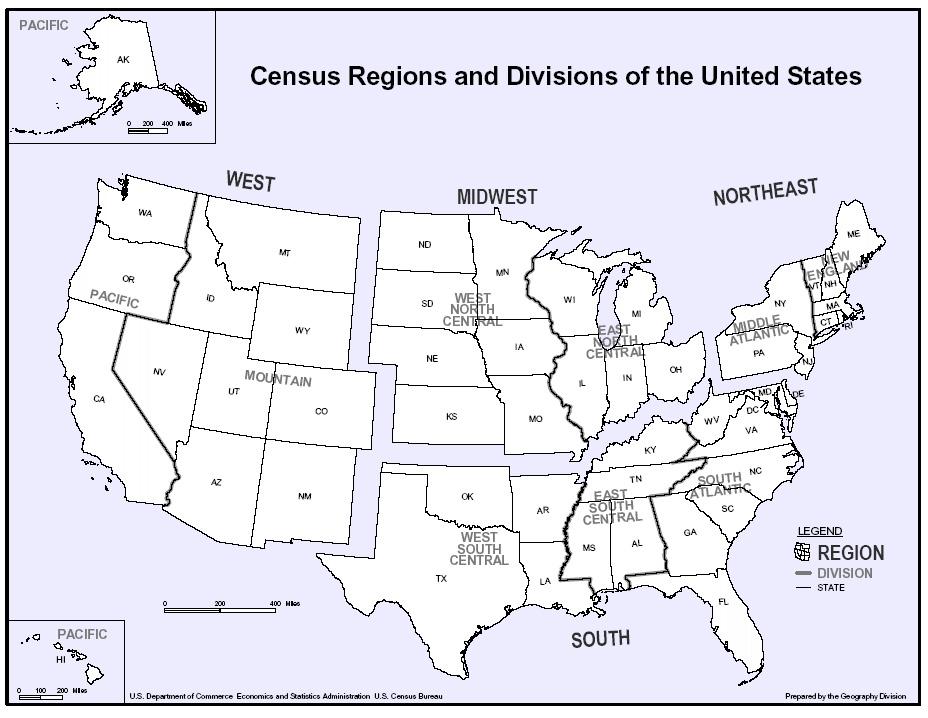
74